EEmc Gammas via conversion method, chi2 comparison
Updated on Thu, 2008-03-20 11:26. Originally created by jwebb on 2008-03-19 14:22.
.png)
.png)
.png)
.png)
EEmc Gammas via conversion method, chi2 comparison
Abstract: Using the conversion method discussed previously, we examine shower-shape variables in greater detail. Specifically, we compare χ2/ndf distributions using shower-shapes derived from MC and from identified η decays.
Method: Shower shapes are determined by summing up single photons from MC events and from identified etas [provide a link]. Three different shower shapes, labeled MC, WILL and PIBERO are studied. For each gamma candidate, we compute a χ2/ndf value using the following procedure:
pseudo-code:
// compute umean and vmean beneath gamma candidate
Float_t chi2 = 0.;
Int_t   ndf  = 0;
for ( int del=-12; del <= +12; del++ )
{
   Float_t shape  = SS[del+12];
   Float_t eshape = SSErr[del+12];
   Float_t uenergy = ustrip[umean+del]->energy;
   Float_t venergy = vstrip[vmean+del]->energy;
   if ( !ufail[umean+del] )
   {
      ndf++;
      chi2 += (uenergy-shape)*(uenergy-shape)/eshape/eshape;
   }
   if ( !vfail[vmean+del] )
   {
      ndf++
      chi2 += (venergy-shape)*(venergy-shape)/eshape/eshape;
   }
}
----
As a reminder, we apply the following cuts in order --
1. Require candidate to be w/in the EEMC with pT > 5.0 GeV.
2. Hadronic veto -- require sum of all postshower tiles w/in R < 0.3 to be less than 0.2 MeV energy deposited.
3. Charged particle veto -- require sum of all preshower-1 tiles w/in R < 0.3 to be == 0
4. Isolation cut -- ET / ETR<0.3 > 0.9
5. Sum of energy deposited w/in preshower-2 > 0 MeV.
And assume efficiencies for cut 5 to be
εgamma = 0.660 +/- 0.013
εbackground = 0.925 +/- 0.054
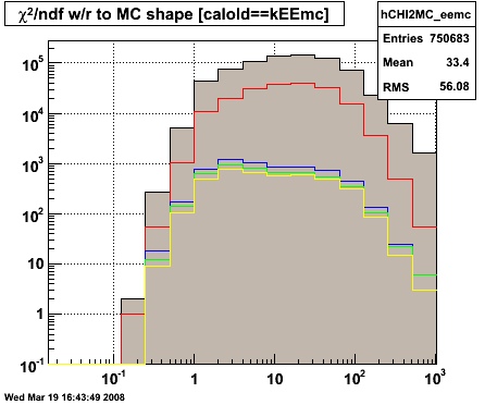
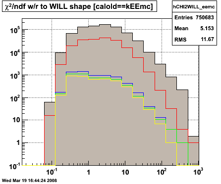
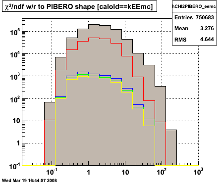
Figure 1 -- Four sub figures showing how (a) the pT distribution evolves with cuts, (b) the MC shower shape χ2/ndf distribution evolves with cuts, (c) Will's shower shape χ2/ndf distribution evolves with cuts and (d) Pibero's shower shape χ2/ndf distribution evolves with cuts. Note logarithmic x-axis on the χ2/ndf distributions.
Figure 2 -- Gamma yields obtained by the conversion method vs (a) pT, (b) the MC shower shape χ2/ndf, (c) Will's shower shape χ2/ndf, and (d) Pibero's χ2/ndf. The solid line indicates all events which passed the isolation cut. The dashed line indicates all events which subsequently deposited energy in the 2nd preshower layer. The blue data points indicate the extracted photon yield. Only statistical errors on the extraction are shown.
How sensitive is the conversion method to systematic uncertaties in the efficiencies? First, examine equation 2 on the conversion method page. It should be fairly obvious that a 1% uncertainty in determining εbackground corresponds to a 1% uncertainty in the photon yield. (Just do a Taylor series expansion in εgamma). So I am not overly concerned that I have neglected the (eta,zvertex) dependance of the gamma efficiency. And I'm not too concerned about the 5-10% difference between Monte Carlo and calculation. Such uncertainties are relevant for a final analysis, but for rough estimates for the BUR we should be fine.
Propagating the uncertainty due to the background efficiency is more complicated, so I take the easy way out. I run the yield extraction code three times. Once with the nominal value of εbackground, and once with εbackground +/- 5.4%.
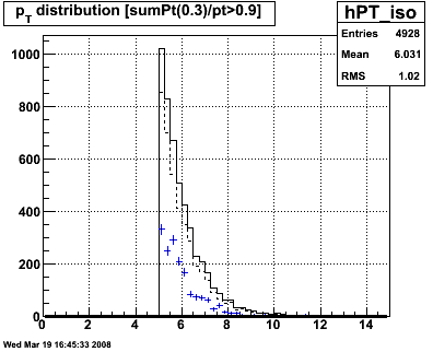
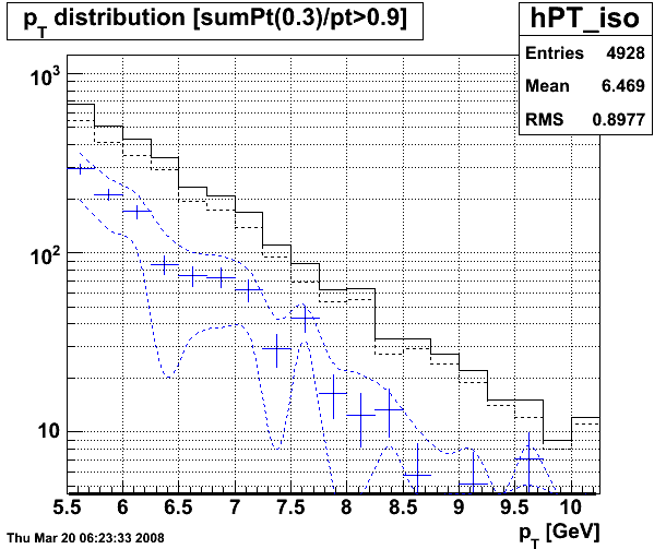
Figure 3 -- pT distribution for gamma candidates above pT = 5.5 GeV. The solid (dashed) black histograms show the events which passed the isolation (2nd preshower) cut. The blue data points show the extracted single gamma yield. The dashed blue lines show the error bands which correspond to a 5.4% uncertainty in determining εbackground.
Here, a 5% uncertainty in the background efficiency corresponds to a +/- 33% uncertainty in our yield estimates.
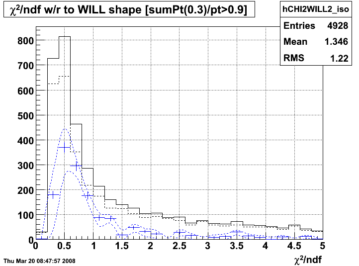
Figure 4 -- chi2/ndf distribution with systematic uncertainties due to a 5.4% uncertainty in background conversion rates.
»
- jwebb's blog
- Login or register to post comments