Run-11 Transverse Jets: PID Update to Spin-PWG (December 21, 2015)
After the Spin-PWG meeting, we developed a final strategy for determining the signal fractions, when using dE/dx. The fit function will utilize five Gaussian peaks: one for each of pions, kaons, protons, electrons, and "merged" tracks (likely pions merged with pile-up tracks). All parameters in the "merged" peak will float. By examining the distributions of nσ(π) vs. nσ(K), nσ(p), and nσ(e), we can fix the separation between the pion centroid and those of K, p, and e. The K and p peaks will share the same width, which will be allowed to float along with that of the e peak. All amplitudes will also float, leaving 11 free parameters in fitting the nσ(π) distribution.
Fixing K, p, and e Centroids
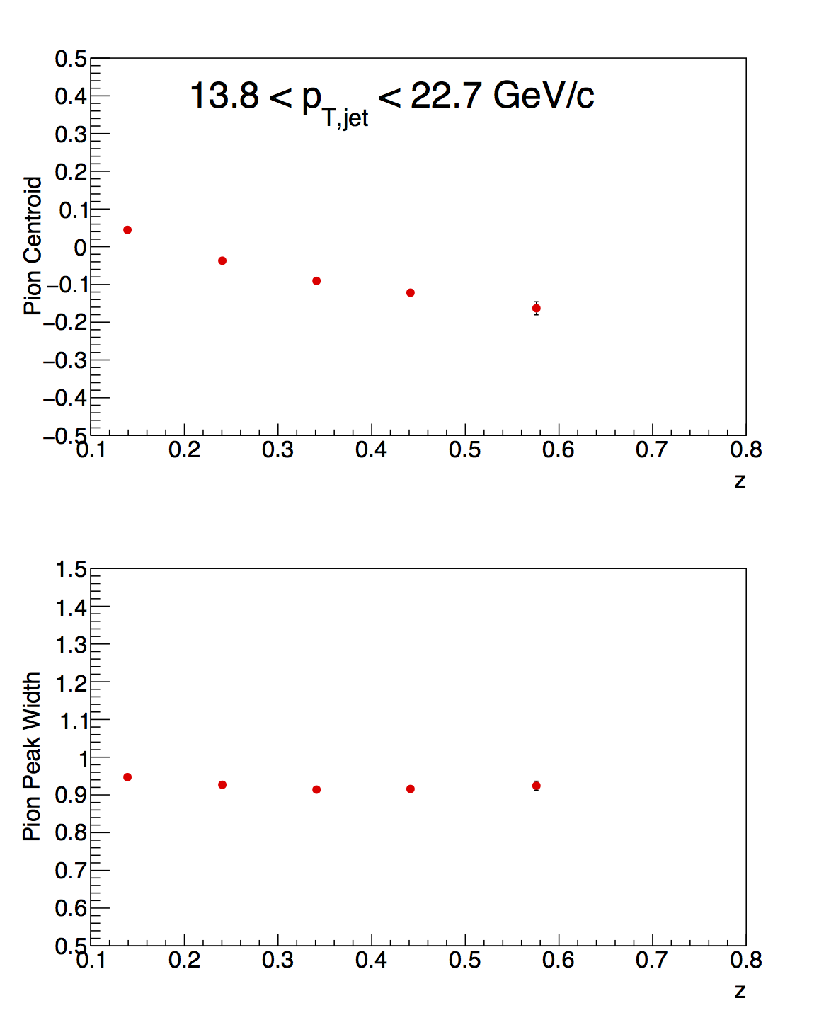
Figures 1-3 present nσ(π) vs. nσ(K), nσ(p), and nσ(e) for z-bins in the three pT ranges. A TProfile overlays the histograms showing the average nσ(π) value for each bin of nσ(K,p,e). The profile is fitted with a 3rd-order polynomial. From the fit, the average nσ(π) value for nσ(K,p,e) = 0 can be found. These values are taken as the separation between the pion peaks and the K, p, and e peaks. The extracted values are presented in Tables 1-3.
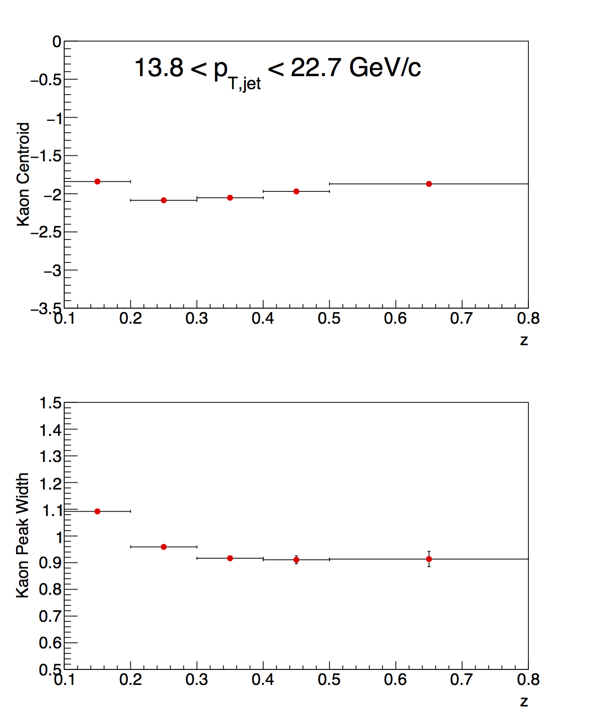
Figure 1: nσ(π) vs. nσ(K)
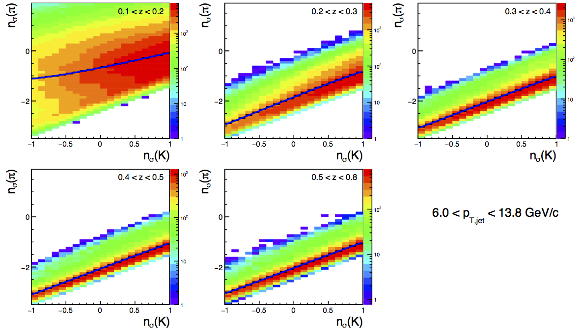
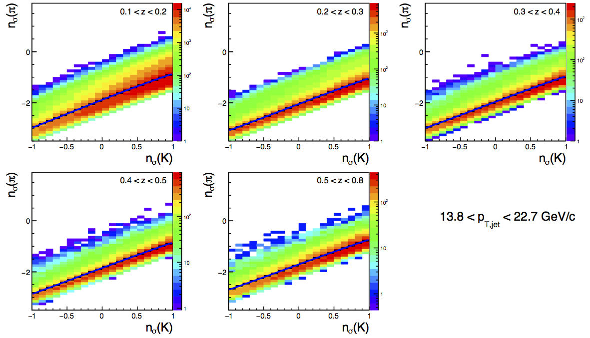
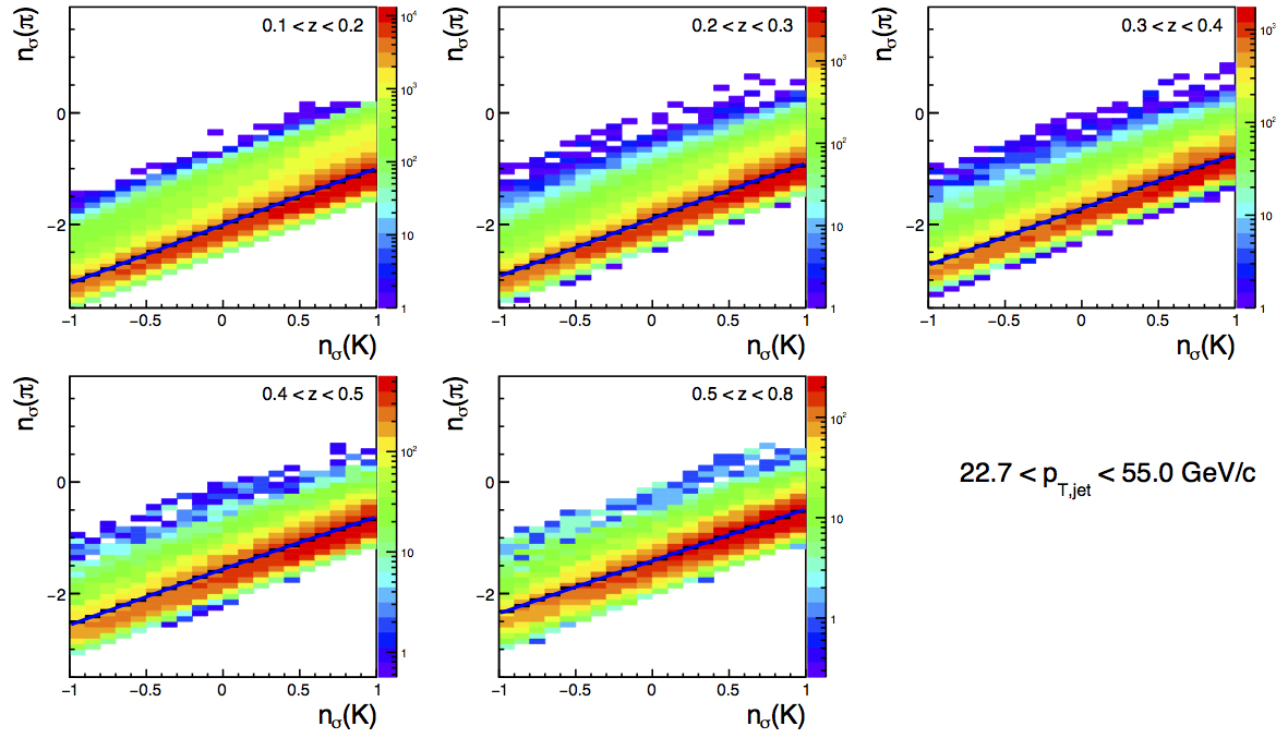
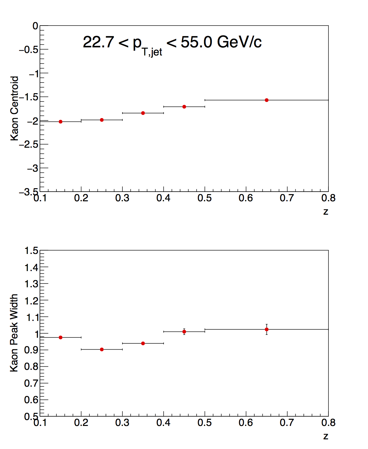
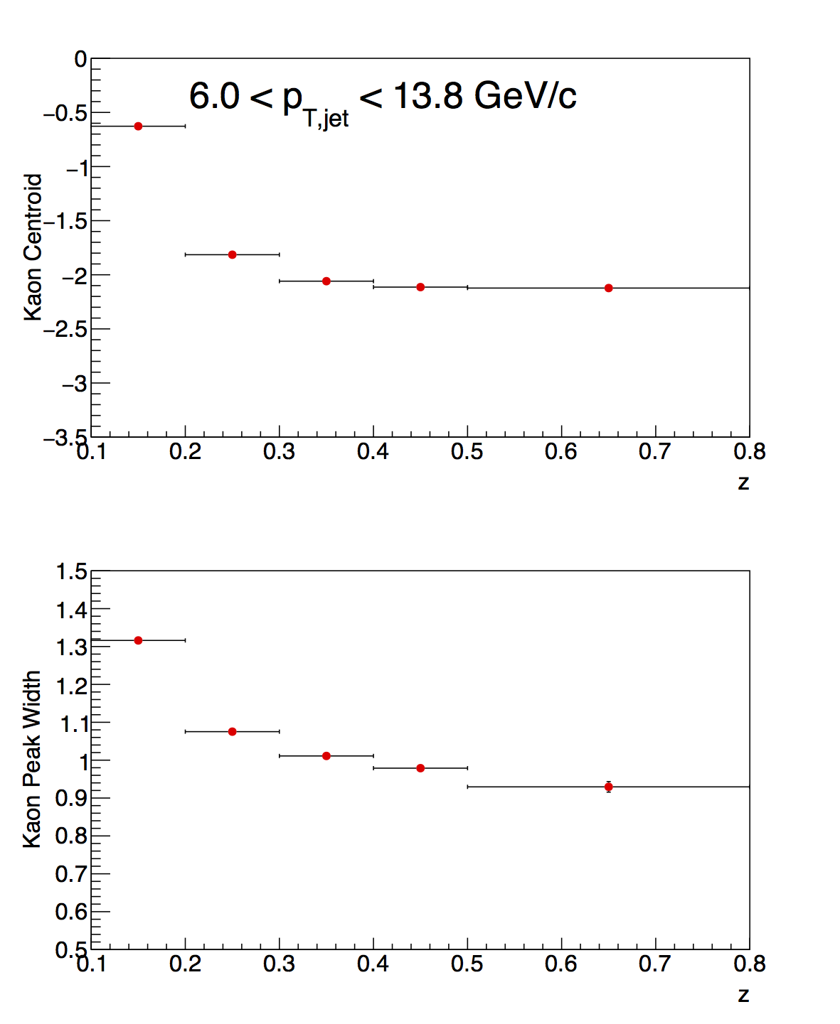
Table 1: Kaon-Pion nσ(π) Separation
| z | Low-pT K-π | Mid-pT K-π | High-pT K-π |
| 0.1-0.2 | -0.676 | -1.885 | -2.009 |
| 0.2-0.3 | -1.848 | -2.049 | -1.896 |
| 0.3-0.4 | -2.034 | -1.962 | -1.715 |
| 0.4-0.5 | -2.069 | -1.848 | -1.562 |
| 0.5-0.8 | -2.036 | -1.708 | -1.412 |
Figure 1 demonstrates quite vividly why nσ(π) does not work for separating kaons and pions at low-z and low-pT. The kaon dE/dx band crosses the pion band in the first z-bin at low pT, where the scatter plot is quite broad and the centroids are separated by less than 1σ. Above the first z-bin at low-pT, the distributions are more focused; and the pion and kaon peaks better separated.
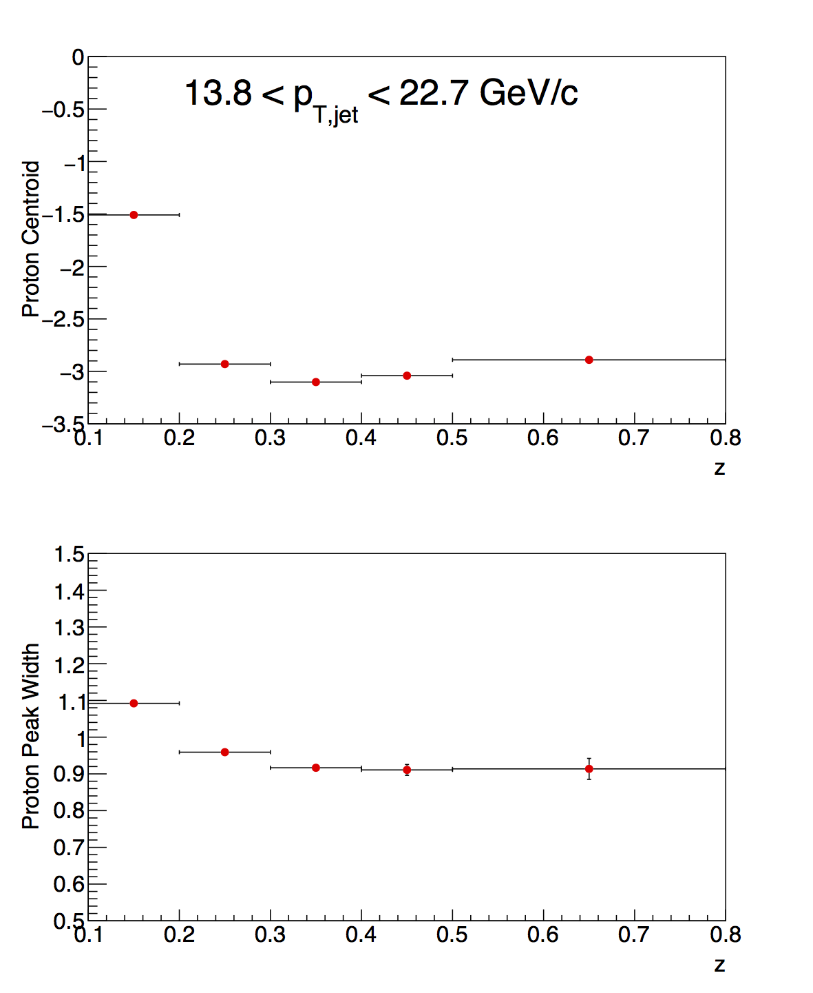
Figure 2: nσ(π) vs. nσ(p)
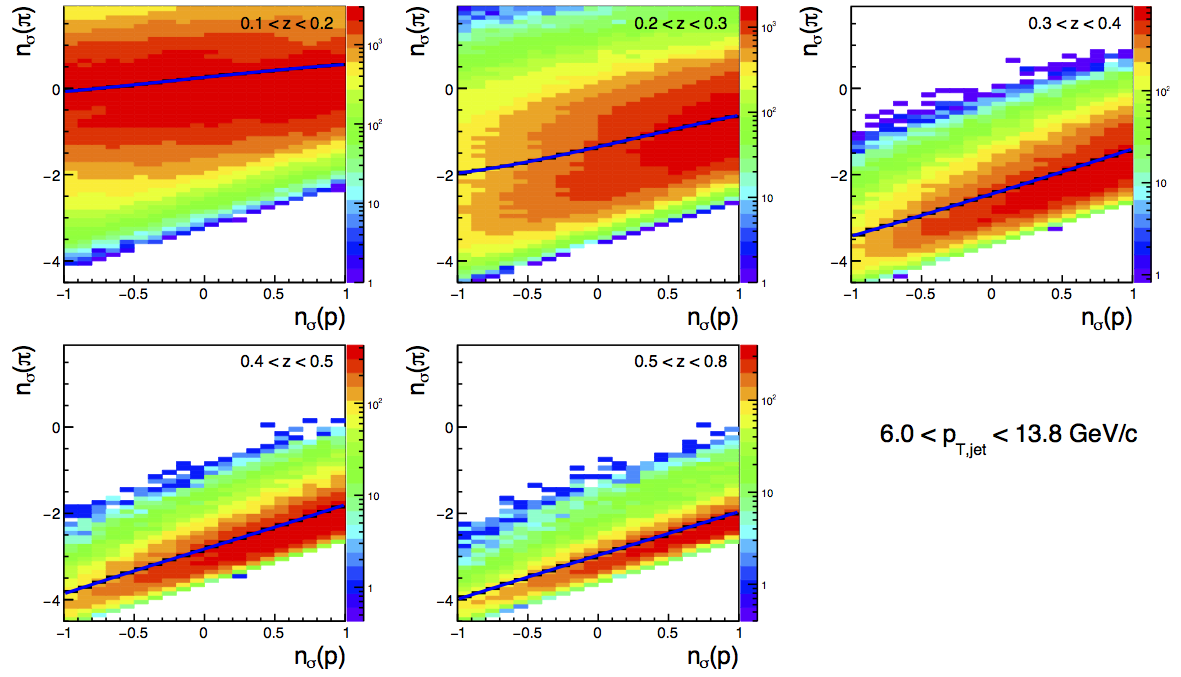

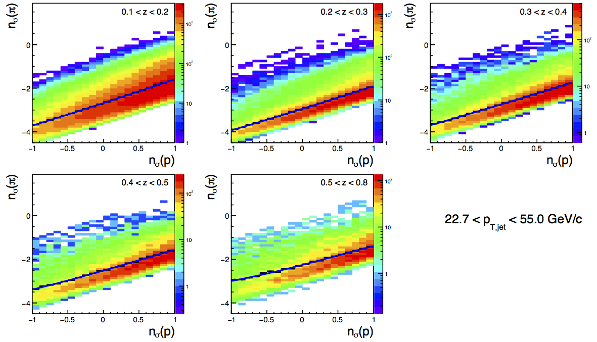
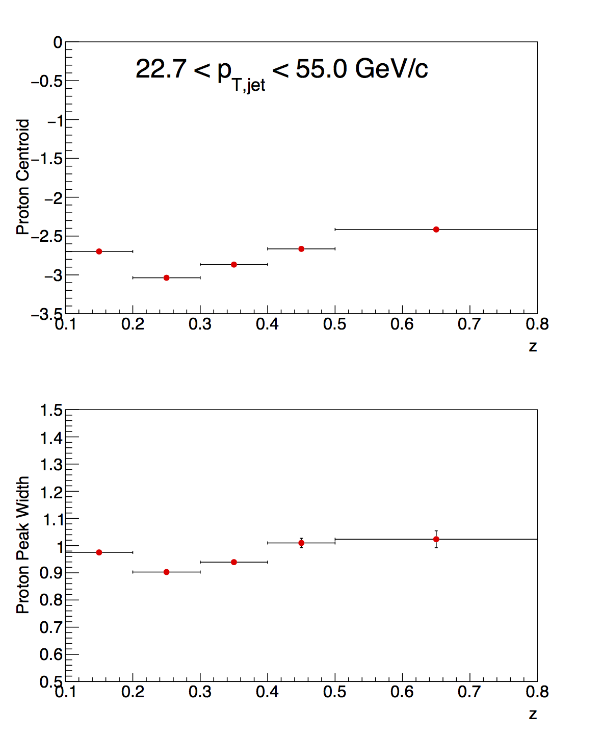
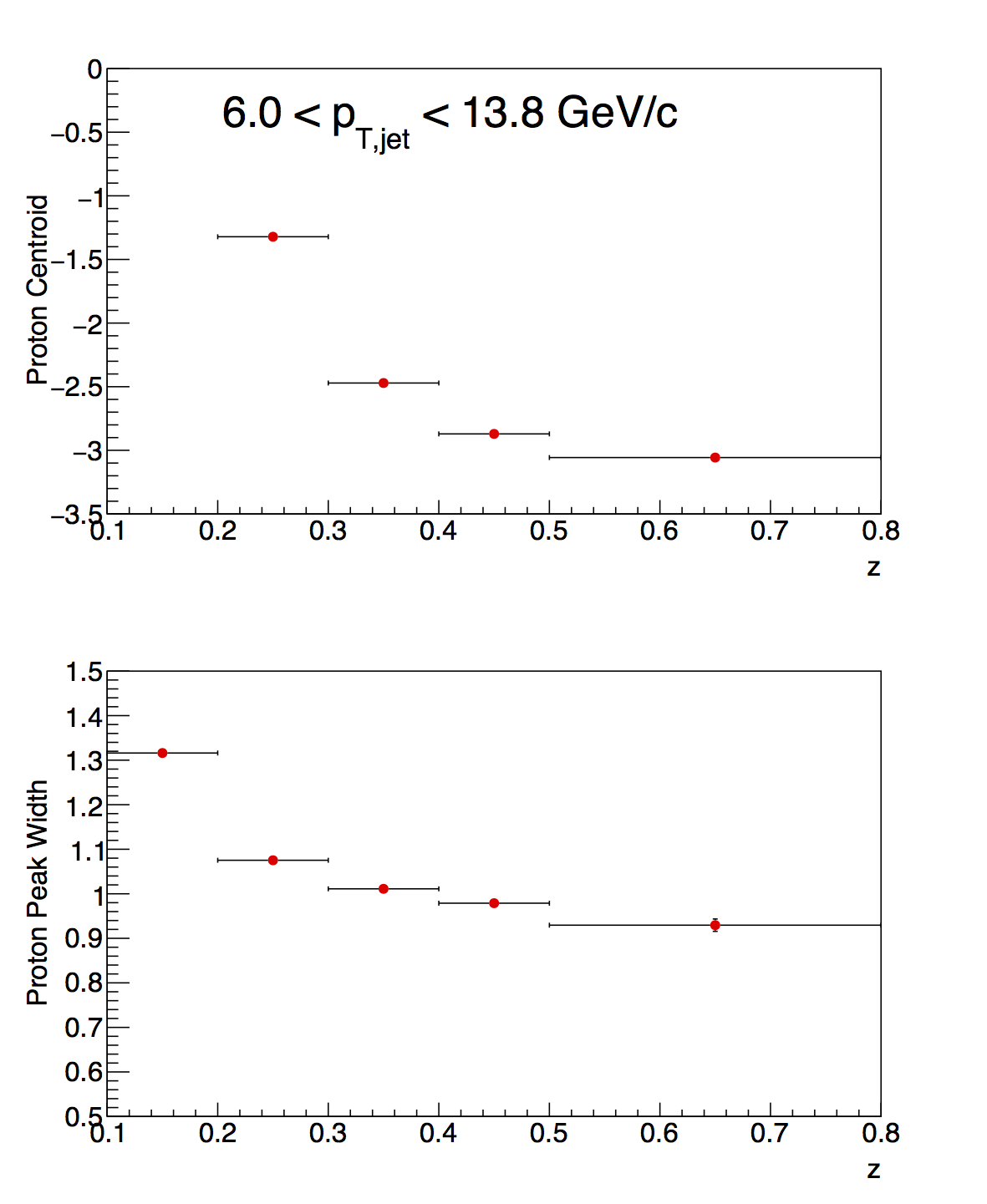
Table 2: Proton-Pion nσ(π) Separation
| z | Low-pT p-π | Mid-pT p-π | High-pT p-π |
| 0.1-0.2 | 0.255 | -1.554 | -2.682 |
| 0.2-0.3 | -1.355 | -2.893 | -2.945 |
| 0.3-0.4 | -2.446 | -3.011 | -2.738 |
| 0.4-0.5 | -2.826 | -2.919 | -2.517 |
| 0.5-0.8 | -2.970 | -2.727 | -2.256 |
Similarly to Fig. 1 in the case of the kaons, Fig. 2 illustrates quite vividly why nσ(π) does not work to separate pions from protons. The proton band crosses the pion band around the second z bin at low-pT. This can be seen in Table 2, as the proton centroid moves from one side of the pion peak to the other. The first two z-bins at low-pT and the first z-bin at mid-pT may have issues in using dE/dx for separating pions from protons. However, in each case, TOF can help.
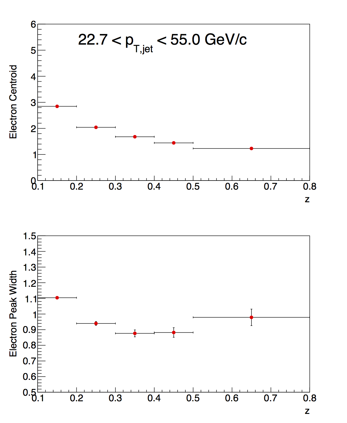
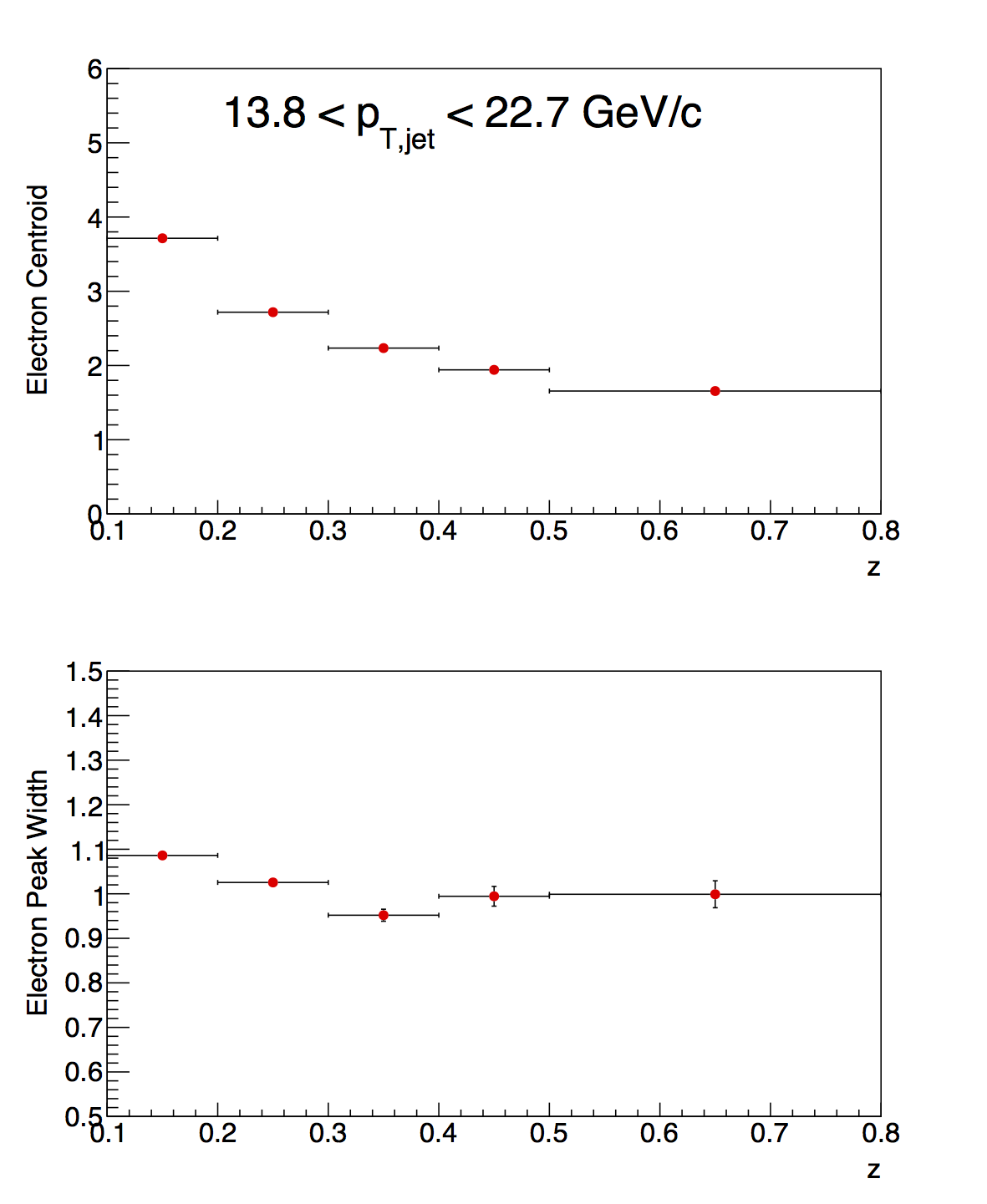
Figure 3: nσ(π) vs. nσ(e)
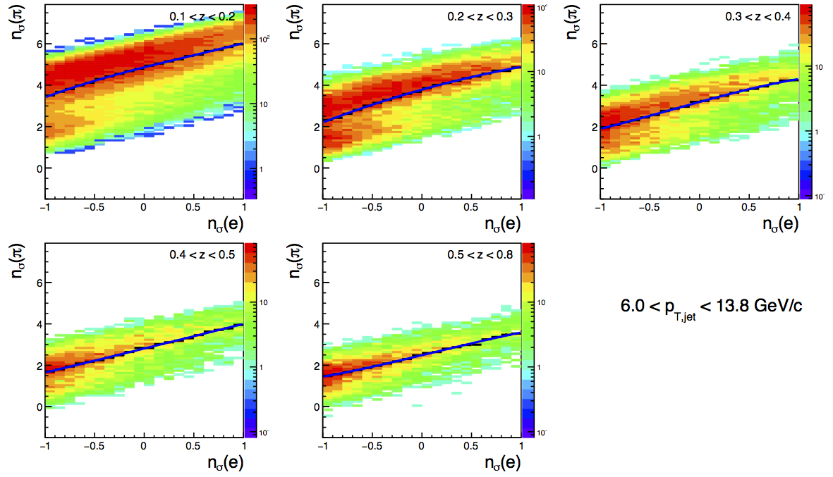
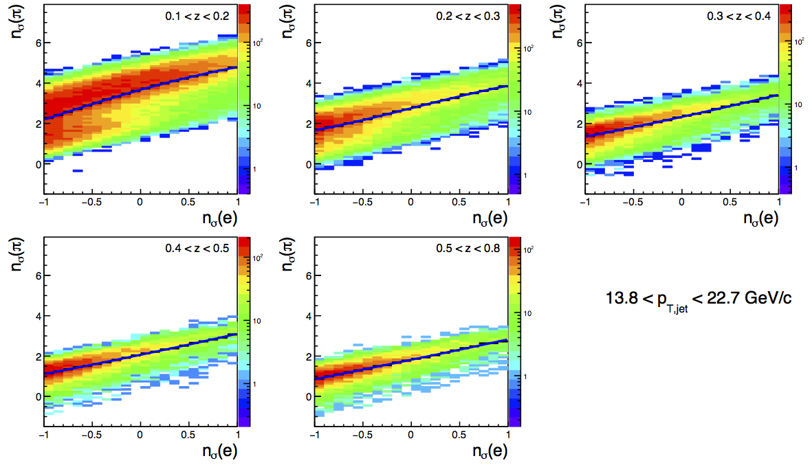
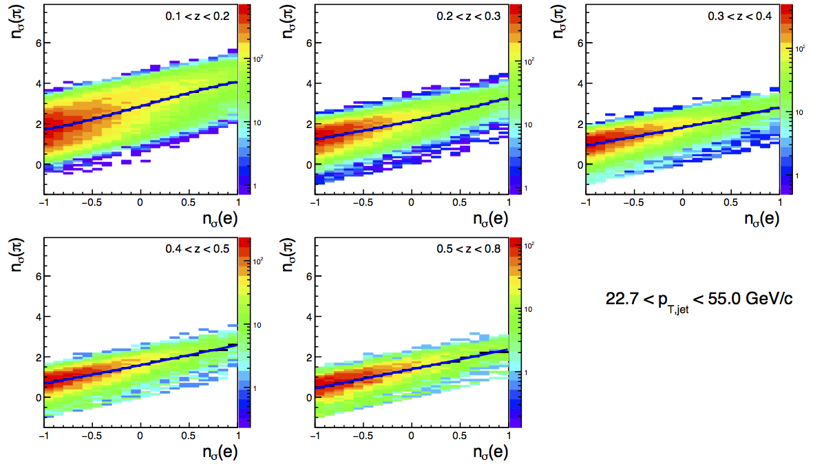
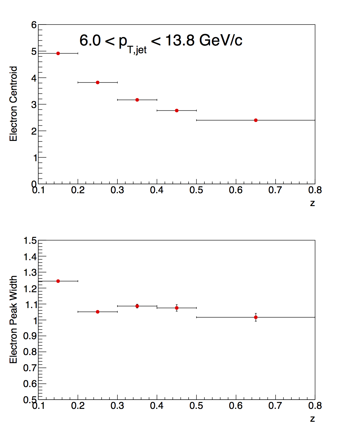
Table 3: Electron-Pion nσ(π) Separation
| z | Low-pT e-π | Mid-pT e-π | High-pT e-π |
| 0.1-0.2 | 4.866 | 3.669 | 2.862 |
| 0.2-0.3 | 3.787 | 2.755 | 2.134 |
| 0.3-0.4 | 3.191 | 2.325 | 1.809 |
| 0.4-0.5 | 2.809 | 2.063 | 1.593 |
| 0.5-0.8 | 2.486 | 1.819 | 1.390 |
Electrons are quite well separated from pions at low-pT and low-z. Where they become an issue is at higher values of z and pT. Fits can become quite unstable under these cases, so being able to fix the centroids to a well-motivated value is tremendously beneficial and a significant improvement over the previous methodology.
Full Fits to nσ(π)
Figure 4: High-pT
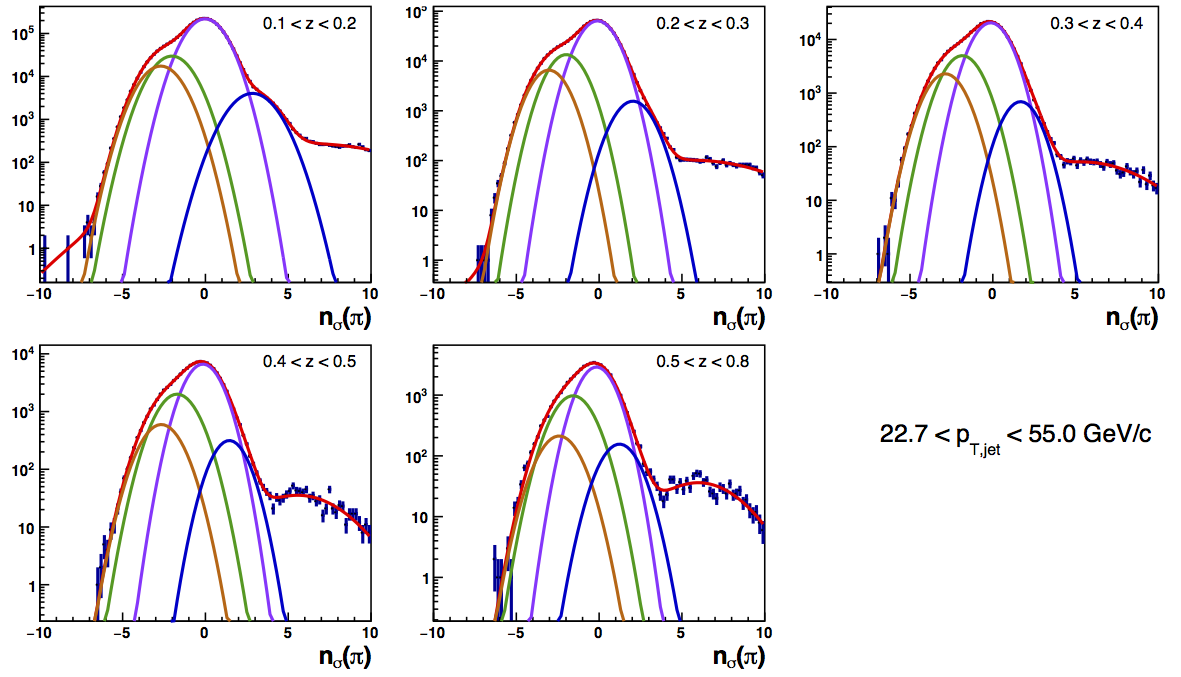
Figure 5: High-pT
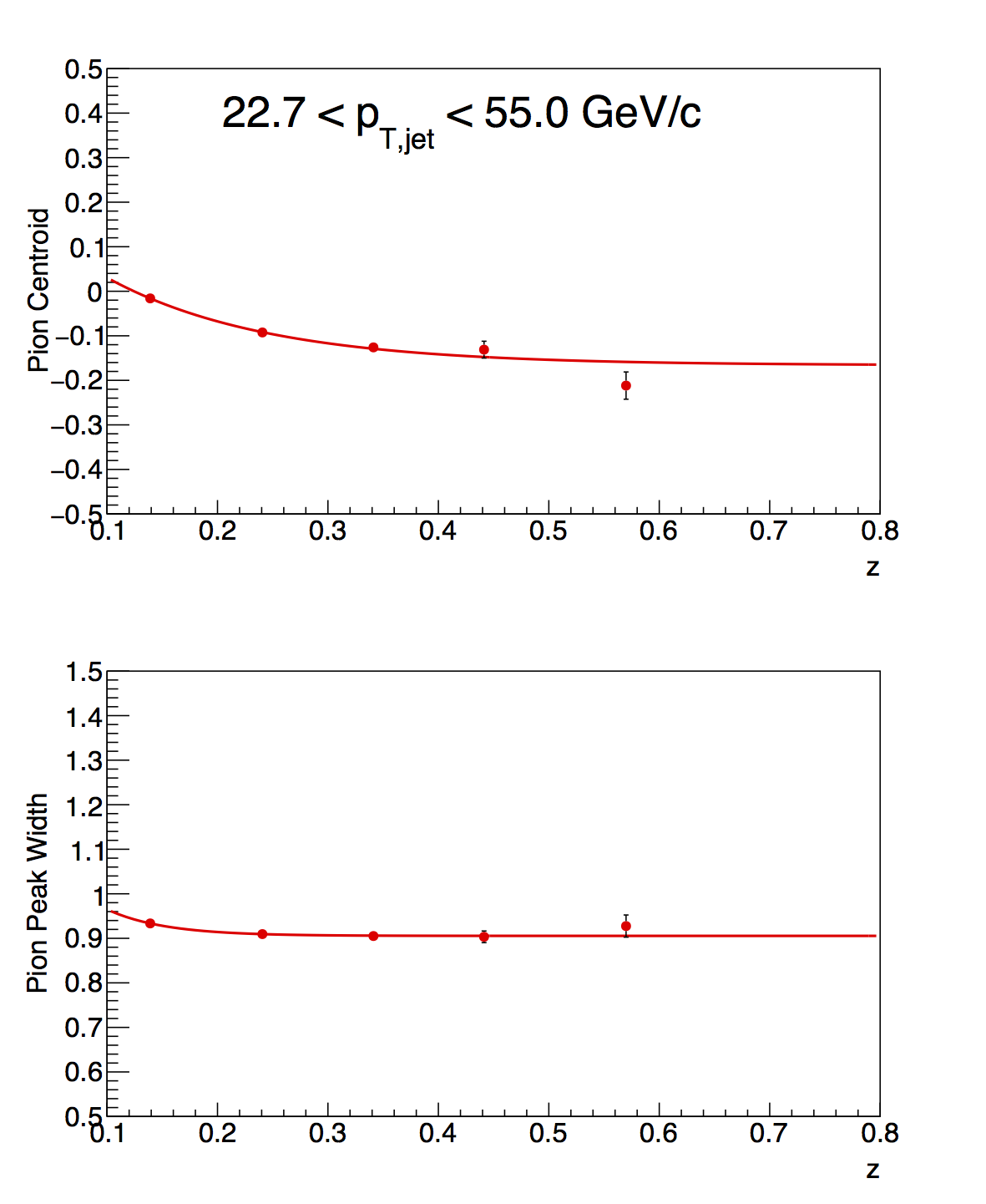
The high-pT fits were done twice. First, the fit was done allowing the pion centroids and widths to float. Once completed, it was observed that they followed an apparently smooth, exponential trend. To tune the fits further, the pion centroids and withers were fitted with an exponential plus constant function and the pion parameters fixed at these values. The fit was redone, and the plots reflect the final fits (save the pion centroids and widths, to illustrate what the values looked like prior to being fixed).
Table 4: High-pT
| -1 < nσ(π) < 2.5 | -4 < nσ(π) < -1.5 | -∞ < nσ(π) < +∞ | ||||||||||
| z | Pion Frac | Kaon Frac | Proton Frac | Elect Frac | Pion Frac | Kaon Frac | Proton Frac | Elect Frac | Pion Yield | Kaon Yield | Proton Yield | Elect Yield |
| 0.1-0.2 | 0.9625 | 0.0235 | 0.0038 | 0.0093 | 0.2547 | 0.4418 | 0.3028 | 4.1×10⁻⁶ | 2.568×10⁶ | 3.640×10⁵ | 2.132×10⁵ | 5.590×10⁴ |
| 0.2-0.3 | 0.9456 | 0.0322 | 0.0014 | 0.0195 | 0.2105 | 0.5014 | 0.2873 | 7.2×10⁻⁶ | 7.289×10⁵ | 1.521×10⁵ | 7.430×10⁴ | 1.838×10⁴ |
| 0.3-0.4 | 0.9144 | 0.0514 | 0.0030 | 0.0297 | 0.2038 | 0.5004 | 0.2953 | 1.5×10⁻⁵ | 2.326×10⁵ | 5.881×10⁴ | 2.697×10⁴ | 7.605×10³ |
| 0.4-0.5 | 0.8655 | 0.0851 | 0.0052 | 0.0428 | 0.2005 | 0.5676 | 0.2318 | 5.7×10⁻⁵ | 7.532×10⁴ | 2.533×10⁴ | 7.547×10³ | 3.481×10³ |
| 0.5-0.8 | 0.8282 | 0.1107 | 0.0070 | 0.0523 | 0.2100 | 0.6000 | 0.1896 | 0.0005 | 3.286×10⁴ | 1.252×10⁴ | 2.724×10³ | 1.914×10³ |
Figure 6: Mid-pT
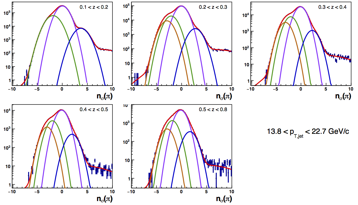
Figure 7: Mid-pT
The 0.1 < z < 0.2 bin at mid-pT fit fails to converge with a nonzero amplitude for the proton peak. This is perhaps not surprising, given that we already expect dE/dx to be unable to separate pions and protons in this bin. Additionally, since the proton band is changing rather quickly in this bin, the Gaussian approximation of the proton peak is probably not a good assumption. Above the 0.1-0.2 bin, the fits converge rather sensibly.
Table 5: Mid-pT
| -1 < nσ(π) < 2.5 | -4 < nσ(π) < -1.5 | -∞ < nσ(π) < +∞ | ||||||||||
| z | Pion Frac | Kaon Frac | Proton Frac | Elect Frac | Pion Frac | Kaon Frac | Proton Frac | Elect Frac | Pion Yield | Kaon Yield | Proton Yield | Elect Yield |
| 0.1-0.2 | 0.9422 | 0.0538 | 2.1×10⁻¹² | 0.0036 | 0.2787 | 0.7210 | 1.6×10⁻¹¹ | 1.1×10⁻⁷ | 3.799×10⁶ | 8.449×10⁵ | 2.276×10⁻⁵ | 9.587×10⁴ |
| 0.2-0.3 | 0.9525 | 0.0304 | 0.0024 | 0.0138 | 0.2018 | 0.5233 | 0.2742 | 2.0×10⁻⁶ | 1.104×10⁶ | 2.320×10⁵ | 1.074×10⁵ | 3.271×10⁴ |
| 0.3-0.4 | 0.9362 | 0.0350 | 0.0014 | 0.0260 | 0.1866 | 0.5377 | 0.2746 | 5.1×10⁻⁶ | 3.517×10⁵ | 8.784×10⁴ | 3.999×10⁴ | 1.344×10⁴ |
| 0.4-0.5 | 0.9125 | 0.0420 | 0.0017 | 0.0425 | 0.1902 | 0.5235 | 0.2850 | 4.2×10⁻⁵ | 1.182×10⁵ | 3.146×10⁴ | 1.449×10⁴ | 6.417×10³ |
| 0.5-0.8 | 0.8840 | 0.0494 | 0.0020 | 0.0634 | 0.2272 | 0.5326 | 0.2388 | 1.8×10⁻⁴ | 5.826×10⁴ | 1.561×10⁴ | 5.502×10³ | 4.275×10³ |
With the possible exception of the kaons, the signal fractions found in the 0.1-0.2 bin should not be believed. Above this bin, the extracted fractions appear to be quite reasonable. In the 0.1-0.2 range, TOF information will give reliable estimates.
Figure 8: Low-pT
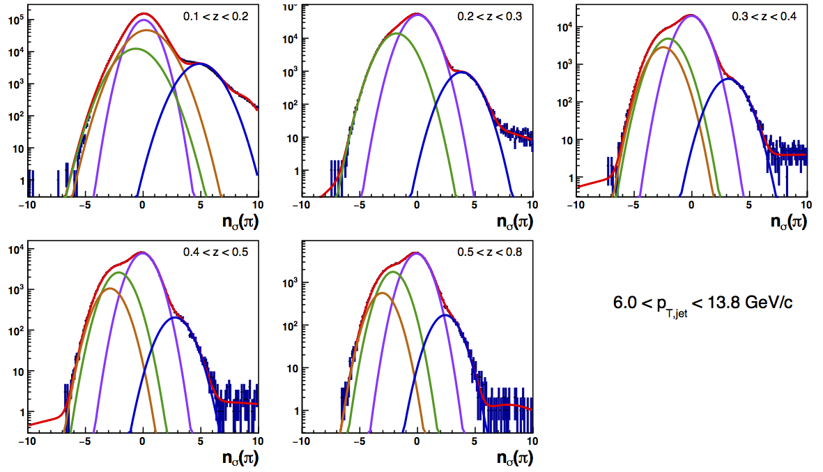
Figure 9: Low-pT
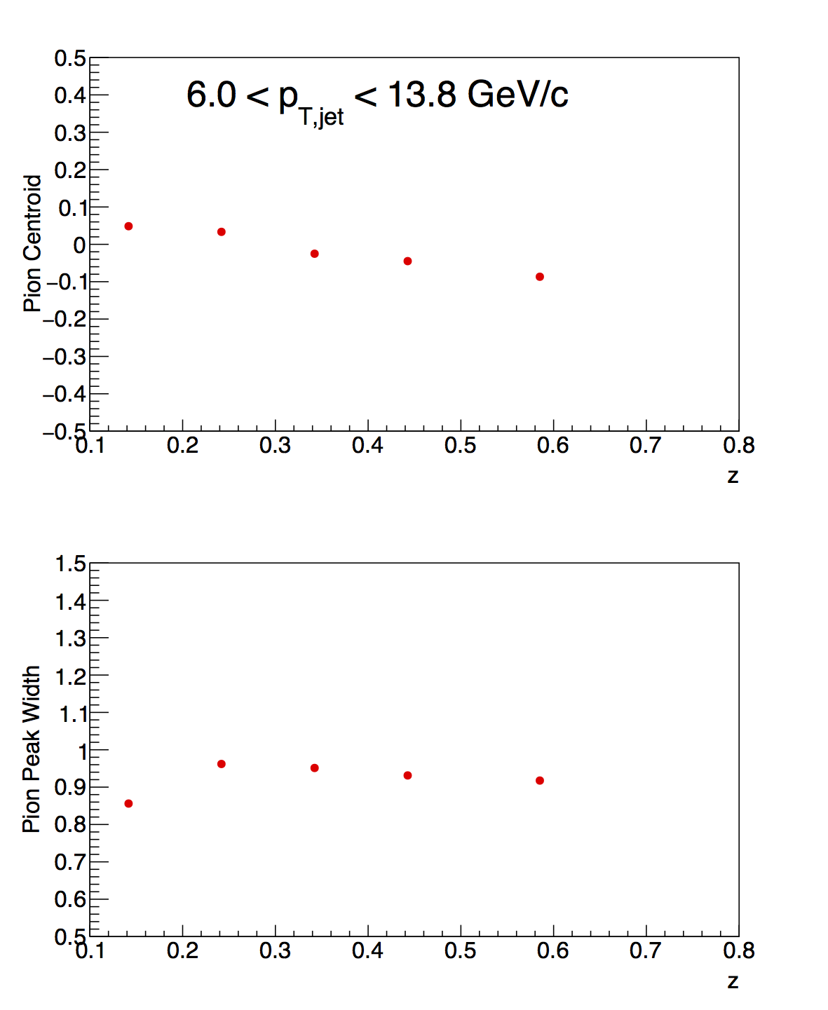
At low-pT, we expect the dE/dx PID to be insufficient to separate pions, kaons, and protons in the 0.1-0.3 range. In fact, we observe the fits in this region to be of rather poor quality. Above the 0.2-0.3 bin, the fits converge rather sensibly.
Table 6: Low-pT
| -1 < nσ(π) < 2.5 | -4 < nσ(π) < -1.5 | -∞ < nσ(π) < +∞ | ||||||||||
| z | Pion Frac | Kaon Frac | Proton Frac | Elect Frac | Pion Frac | Kaon Frac | Proton Frac | Elect Frac | Pion Yield | Kaon Yield | Proton Yield | Elect Yield |
| 0.1-0.2 | 0.5588 | 0.0738 | 0.3664 | 0.0010 | 0.2415 | 0.3312 | 0.4273 | 5.3×10⁻⁸ | 2.099×10⁶ | 4.081×10⁵ | 1.543×10⁶ | 1.308×10⁵ |
| 0.2-0.3 | 0.9228 | 0.0745 | 1.2×10⁻¹¹ | 0.0023 | 0.2330 | 0.7667 | 5.4×10⁻¹¹ | 1.8×10⁻⁸ | 1.228×10⁶ | 3.772×10⁵ | 3.7×10⁻⁵ | 2.464×10⁴ |
| 0.3-0.4 | 0.9366 | 0.0433 | 0.0126 | 0.0072 | 0.1677 | 0.5003 | 0.3317 | 5.9×10⁻⁷ | 4.635×10⁵ | 1.226×10⁵ | 7.239×10⁴ | 1.120×10⁴ |
| 0.4-0.5 | 0.9317 | 0.0499 | 0.0044 | 0.0136 | 0.1392 | 0.5916 | 0.2688 | 2.6×10⁻⁶ | 1.805×10⁵ | 6.402×10⁴ | 2.590×10⁴ | 5.502×10³ |
| 0.5-0.8 | 0.9267 | 0.0476 | 0.0018 | 0.0239 | 0.1423 | 0.6350 | 0.2227 | 5.8×10⁻⁶ | 1.089×10⁵ | 4.130×10⁴ | 1.320×10⁴ | 4.367×10³ |
Again, the fractions and yields for pions, protons, and kaons are suspect in the region of 0.1-0.3 (perhaps the kaons are okay in the 0.2-0.3 bin, to be determined). Above this, however, the information is rather sensible. The 0.1-0.3 region will rely on information from TOF.
- drach09's blog
- Login or register to post comments