Run 8 BTOW Calibration (2008)
2008 BTOW calibrations
- BTOW HV used in 2008 are in the file 2008_i2a.csv, this file will contain a few towers
(<50)which might have been set to zero at a later date
01 statistical analysis of 2008 HV
Goal: study eta dependence of 2008 BTOW HV
Fig 1 Eta-phi distribution of HV

Formulas used to map tower ID in to eta-phi location
    int id0=id-1;
    int iwe=0; // West/East switch
    if(id>2400) iwe=1;
    int id0=id0%2400;
    int iphi=id0/20;
    int ieta=id0%20;
    if(iwe==0) ieta=ieta+20;
    else ieta=19-ieta;
Fig 2 Batch 1, Eta-phi distribution of HV

eta=0.05  mean HV=821 +/- 5  sigHV=60
eta=0.15  mean HV=820 +/- 5  sigHV=60
eta=0.25  mean HV=815 +/- 5  sigHV=62
eta=0.35  mean HV=811 +/- 5  sigHV=66
eta=0.45  mean HV=817 +/- 5  sigHV=66
eta=0.55  mean HV=820 +/- 5  sigHV=57
eta=0.65  mean HV=820 +/- 5  sigHV=59
eta=0.75  mean HV=806 +/- 5  sigHV=62
eta=0.85  mean HV=807 +/- 5  sigHV=58
eta=0.95  mean HV=829 +/- 5  sigHV=65
Fig 3 Batch 2, Eta-phi distribution of HV

eta=0.05  mean HV=759 +/- 6  sigHV=56
eta=0.15  mean HV=760 +/- 7  sigHV=62
eta=0.25  mean HV=756 +/- 6  sigHV=53
eta=0.35  mean HV=763 +/- 6  sigHV=55
eta=0.45  mean HV=756 +/- 7  sigHV=58
eta=0.55  mean HV=760 +/- 6  sigHV=54
eta=0.65  mean HV=743 +/- 6  sigHV=52
eta=0.75  mean HV=754 +/- 6  sigHV=54
eta=0.85  mean HV=754 +/- 7  sigHV=64
eta=0.95  mean HV=769 +/- 7  sigHV=59
Fig 4 Batch 3, Eta-phi distribution of HV

eta=-0.95  mean HV=730 +/- 4  sigHV=57
eta=-0.85  mean HV=723 +/- 4  sigHV=57
eta=-0.75  mean HV=727 +/- 4  sigHV=59
eta=-0.65  mean HV=718 +/- 4  sigHV=58
eta=-0.55  mean HV=723 +/- 4  sigHV=58
eta=-0.45  mean HV=720 +/- 4  sigHV=56
eta=-0.35  mean HV=727 +/- 4  sigHV=54
eta=-0.25  mean HV=724 +/- 4  sigHV=60
eta=-0.15  mean HV=735 +/- 4  sigHV=59
eta=-0.05  mean HV=729 +/- 4  sigHV=60
02 BTOW swaps ver=1.3
Example of MIP peak for BTOW towers pointed by TPC MIP track:  Spectra for 4800 towers (raw & MIP) are in attachment 1.
Method of finding MIP signal in towers:

Table 1
BTOW swaps, very likely, ver 1.3, based on 2008 pp data, fmsslow-production
 266 --> 286 , 267 --> 287 , 286 --> 266 , 287 --> 267 , 389 --> 412 ,
 390 --> 411 , 391 --> 410 , 392 --> 409 , 409 --> 392 , 410 --> 391 ,
 411 --> 390 , 412 --> 389 , 633 --> 653 , 653 --> 633 , 837 --> 857 ,
 857 --> 837 ,1026 -->1046 ,1028 -->1048 ,1046 -->1026 ,1048 -->1028 ,
1080 -->1100 ,1100 -->1080 ,1141 -->1153 ,1142 -->1154 ,1143 -->1155 ,
1144 -->1156 ,1153 -->1141 ,1154 -->1142 ,1155 -->1143 ,1156 -->1144 ,
1161 -->1173 ,1162 -->1174 ,1163 -->1175 ,1164 -->1176 ,1173 -->1161 ,
1174 -->1162 ,1175 -->1163 ,1176 -->1164 ,1753 -->1773 ,1773 -->1753 ,
2077 -->2097 ,2097 -->2077 ,3678 -->3679 ,3679 -->3678 ,3745 -->3746 ,
3746 -->3745 ,4014 -->4054 ,4015 -->4055 ,4016 -->4056 ,4017 -->4057 ,
4054 -->4014 ,4055 -->4015 ,4056 -->4016 ,4057 -->4017 ,4549 -->4569 ,
4569 -->4549 ,
Details for all swaps are shown in attached 2.
Other problems found during analysis, not corrected for, FYI

03 MIP peak analysis (TPC tracks, 2008 pp data)
I examined runs from 2008 pp (list attached below) to create calibration trees (using StRoot/StEmcPool/StEmcOfflineCalibrationMaker). The code loops over the primary tracks in the event and selects the global track associated with it, if available. If the track can be associated to a tower and has outermomentum > 1 GeV, it is saved.
I then loop over those tracks and choose ones that fall within a certain criteria:
- p > 1
- adc - ped > 1.5 * ped_rms
- tower_entrance_id = tower_exit_id
- only a single track points to the tower
- neighoring towers have small amounts of energy
We can sum over all runs to produce MIP spectrum in 4445 towers. Of those, 4350 pass current QA requirements. An example MIP spectrum with fit is shown below. All MIP peaks can be seen in the attached PDF. It's important to note that the uncertainty on the MIP peak location with these statistics is on average 5%. This number is a lower limit on the calibration coefficient uncertainty that can only be improved with statistics.
Fig 1. Typical MIP peak. Plots like this for all 4800 towers are in attachment 1.
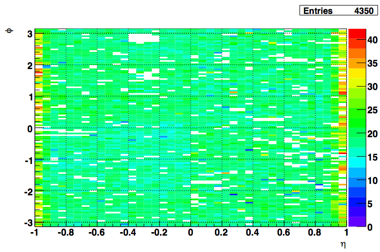
The following plot shows MIP peak location in ADCs (in eta, phi space) of all of towers where such a peak could be found.
Fig 2. MIP Peak (Z-axis) for all towers
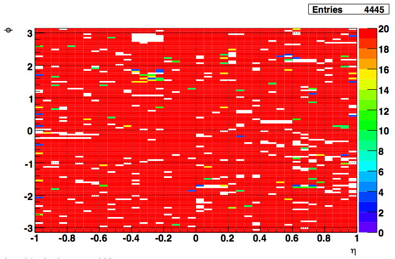
This plot shows the status codes of the towers. White are the towers that had 0 entries in their histograms. Red are the good towers (pushed them off scale to see the rest of the entries). Towers in the outermost eta bin received different treatment. The fit range was between [6,100] for those towers (vs [6,50] for the rest). The cuts applied for QA were slightly loosened. The rest of the codes follow this scheme:
- bit 1: entries in histogram > 0
- bit 2: sigma of fit below threshold (15,20)
- bit 4: mean of fit above 5 ADCs
- bit 8: difference of fit mean and MPV in fit range below threshold (5,10)
Fig 3. status of towers
Spectra of towers rejected by rudimentary automatic QA were manually inspected and 91 were found to contain reasonable MIP peak and have bin re-qualified as good. PLots for those towers are in attachment 2.
04 relative tower gains based on MIPs (gain correction 1)
Determination of relative gains BTOW gains based on MIP peak for the purpose of balancing HV for 2009 run
Procedure:
- use fitted 03 MIP peak analysis (TPC tracks, 2008 pp data)
- find average MIP value for 40 eta bins
- West barrel: preserve absolute average MIP peak position in the , compute gain correction to equalize all towers at given eta to the average for this eta
- East barrel: enforce absolute average MIP peak to agree with the West barrel, correct relative gains in the similar way.
In this stage of calibration process 4430 towers with well visible MIP peak were use. The remaining 370 towers will be called 'blank towers' . There are many reasons MIP peak doe snot show up e.g. dead hardware. ~60 of the 'blank towers' are 02 BTOW swaps ver=1.3- as identified earlier and not corrected in this analysis.
Fig 1. Left: MIP peak (Z-axis) was found for 4430 towers shown in color. White means no peak was found - those are "blank towers". Right: eta-phi distribution of blank towers. On both plots East (West) barrel is show on etaBins [1-20], (21,40).

The (iEta, iPhi ) coordinates were computed based on softID as follows:
   int jeta= 1+(id-1)%20; // range [1-20]
   int jphi= 1+(id-1)/20; // range [1-240]
   if(jphi<=120) { // West barrel
      keta=jeta+20; kphi=jphi;
   } else { // East barrel
      keta=-jeta+21; kphi=jphi-120;
   }
Fig 2. Average MIP position as function of eta bin. West-barrel gains are higher even of average.

Gain corrections (GC1) were computed as
GC1(iEta,iPhi)= MIP(iEta,iPhi) / avrMip(iEta)
For the East-barrel we used values of avrMip(iEta)from symmetric eta-bins from the West barrel.
If computed correction was between [0.95,1.05] or if towers was "blank" GC1=1.00 was used.
Fig 3. Left distribution of gain corrections GC1(iEta). Right: value of GC1(iEta,iPhi).

Attached spreadsheet contains computed GC1(softID) in column 'D' together with MIP peak parameters (columns H-P) for all 4800 towers. Below is just first 14 towers.

Used .C macro is attached as well.
05 Absolute Calibration from Electrons
We use the MIP ADC location calculated in part 03 to get a preliminary measure of the energy scale for each tower.
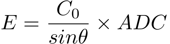
The following formula from SN436 provides the calibration coefficient:
C = 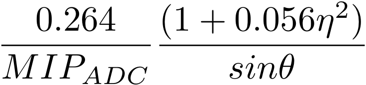
where E = C * (ADC - ped).
For the electron sample I select tracks with:
- 1.5 < p < 6.0 (GeV)
- dR < 0.0125 (from center of face of tower in eta/phi space)
- adc - ped > 2.5 * ped_rms in tower
- nHits > 10
- nSigmaElectron > -1
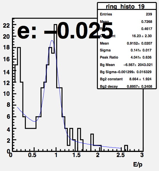
Here is one of the E/p distributions. Note the error on the mean is about 2%, which is about average.
For each electron we calculate E/p and sum over eta rings. Here is the peak of E/p for each eta bin. The error bars show the error on the mean value, and the shaded bar is the sigma. I fit over the range [-0.9,0.0] and [0.0,0.9] separately. The fit for the east reports the mean is 0.9299 +/- 0.0037. For the west, I get 0.9417 +/- 0.0035.
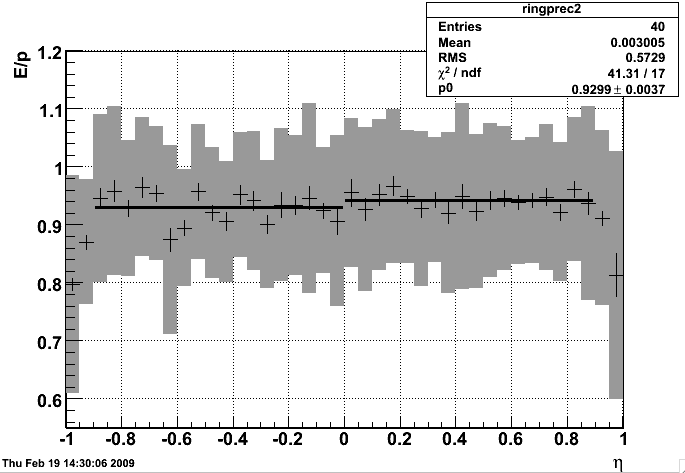
The location of the E/p peak tells us the correction that needs to be applied to the calibration coefficients of towers in each eta ring to get the correct absolute energy.
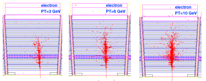
Reference plot (electron showers):
06 Calculating 2009 HV from Electron Calibrations
The ideal gain for each tower satisfies the following relation, where E_T = 60 GeV when ADC is max scale (~4095 - ped):
(1)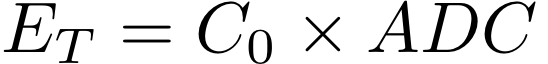
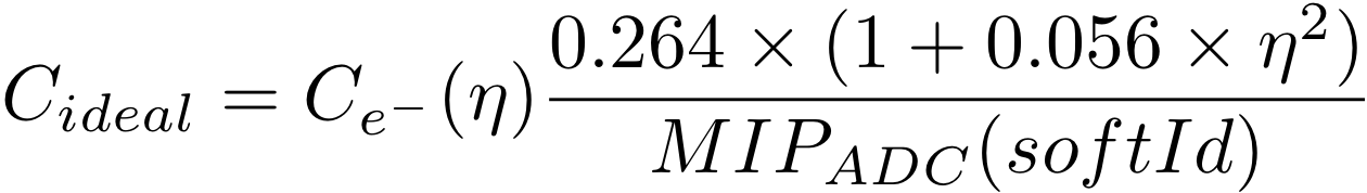
We want to calculate the total energy deposited in a tower, which is the following in the ideal case:
(2)
In reality, we calculate the calibration according to the following formula:
(3)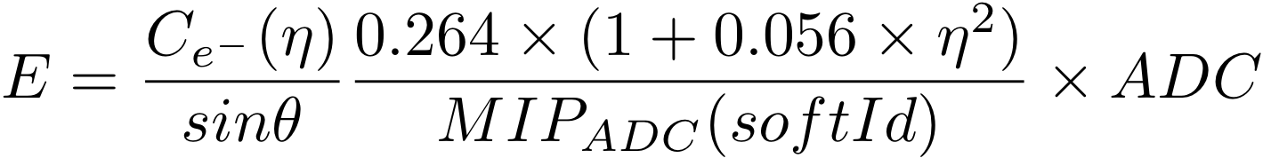
where there is an electron correction for each eta ring, and the MIP location is determined for all towers.
Thus, to have ideal gains, we want the following relation to hold
 (4)
(4)
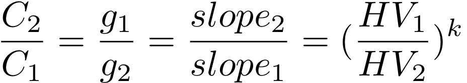
To make this relation true, we need to adjust the high voltage for each tower according to the following relation:
(5)
We can check the changes using slopes.
07 BTOW absolute gains 'ab initio'
Summary of intended BTOW HV change, February 24, 2009
Conclusion:
We will NOT change average gain of West BTOW for eta bins[1,18]. For all other eta bins we will aim at the average West Btow marked as red dashed line.

Full presentation is in attachment 1.
Detailed E/P spectra for 40 eta bins are in attachment 2 & 3.
08 Completed Calibration and Uncertainty
The 2008 Calibraton has been uploaded into the database. I was able to find calibration coefficients for 4420 towers. Of the remaining towers, 353 were MIPless and 27 had spectrums that I could not recover by hand.
This year, differently from previous years, known sources of bias are removed. If an event had a nonHT trigger, the tracks from that event were used for the calibration (even if it had an HT trigger). Most of the triggers were fms slow triggered events. Each eta ring was calibrated separately, and then a correction for each crate was applied. After these corrections, I once again made the cuts on the electrons more stringent. No deviation from E/p =1 was found. With the biases eliminated, we now quote a systematic variance instead of a systematic bias as the uncertainty on the calibration.
The source of this uncertainty are the uncertainties on various fits used for each calibration, namely the MIP peak for each tower, the absolute calibration for each eta ring, and the correction for each crate. These uncertainties are highly correlated. I have completed this calibration by recalculating the calibration table 3,000 times varying the MIP peaks, the eta ring corrrections and the crate corrections each time. Using this method, I was able to determine the correlated uncertainty for each calibrated tower. This uncertainty is, on average, 5%.
This uncertainty is different than the systematic bias quoted for 2005 and 2006. It is a true variance on the calibration. To use this uncertainty, analyzers should recalculated their analysis using test tables generated for this purpose. The variance in the results of these multiple analyses will give a direct measure of the uncertainty due to the calibration scale uncertainty. These tables will be uploaded to the database with the names "sysNN". They should be used before clustering, jet finding, etc.