09 Sep
September 2008 posts
2008.09.02 Shower shape fits
Ilya Selyuzhenkov September 02, 2008
Data sets:
- pp2006 - STAR 2006 pp longitudinal data (~ 3.164 pb^1) after applying gamma-jet isolation cuts.
- gamma-jet - data-driven Pythia gamma-jet sample (~170K events). Partonic pt range 5-35 GeV.
- QCD jets - data-driven Pythia QCD jets sample (~4M events). Partonic pt range 3-65 GeV.
Shower shape fitting procedure:
- Fit with single Gaussian shape using 3 highest strips
- Fit with double Gaussian using 5 strips from each side of the peak [11 strips total]
First Gaussian parameters are fixed from the step above - Re-fit with double Gaussian with initial parameters from step 2 above
- Fit with triple Gaussian [fit range varies from 9 to 15 strips, default is 12 strips, see below]
Initial parameters for the first two Gaussian are fixed from step 3 above - Fit with triple Gaussian with initial parameters from step 4 above
(releasing all parameters except mean values)
Fitting function "[0]*(exp ( -0.5*((x-[1])/[2])**2 )+[3]*exp ( -0.5*((x-[4])/[5])**2 )+[6]*exp ( -0.5*((x-[7])/[8])**2 ))"
Fit results for MC gamma-jet data sample
Figure 1: MC gamma-jet shower shapes and fits for u-plane
Results from single, double and triple Gaussian fits (using from 9 to 15 strips) are shown.
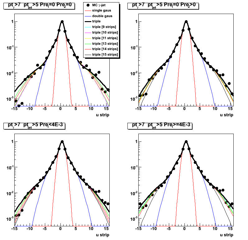
Figure 2: Same as figure 1. but from v-plane
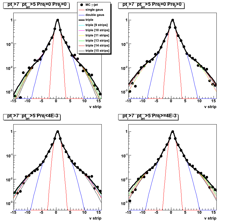
Figure 3: MC gamma-jet results using triple Gaussian fits within 12 strips from a peak.
Left: u-plane. Right: v-plane
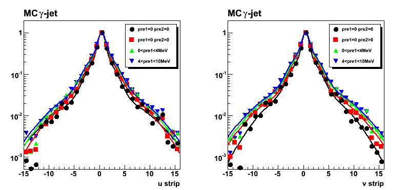
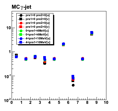
Figure 4: Combined fit results from MC gamma-jet sample
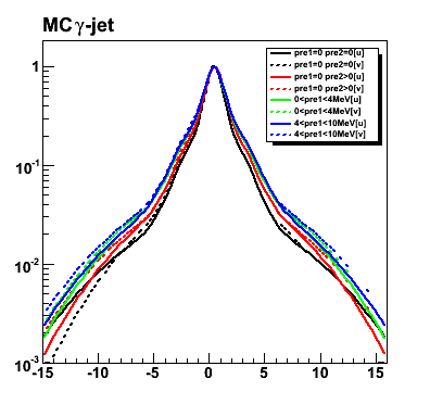
Figure 5: Fitting parameters [see equation for the fit function above].
Note, that parameters 1, 4, and 7 (peak position) has the same value.
Numerical fit results:
- pre1=0 pre2=0 [u]: 0.602039*((exp(-0.5*sq((x-0.491324)/0.605927))+(0.578161*exp(-0.5*sq((x-0.491324)/2.05454))))+(0.0937517*exp(-0.5*sq((x-0.491324)/6.37656))))
- pre1=0 pre2=0 [v]: 0.729744*((exp(-0.5*sq((x-0.480945)/0.621631))+(0.327792*exp(-0.5*sq((x-0.480945)/2.01717))))+(0.0410935*exp(-0.5*sq((x-0.480945)/6.49599))))
- pre1=0 pre2>0 [u]: 0.725212*((exp(-0.5*sq((x-0.474451)/0.560416))+(0.3332*exp(-0.5*sq((x-0.474451)/1.91957))))+(0.0611053*exp(-0.5*sq((x-0.474451)/5.34357))))
- pre1=0 pre2>0 [v]: 0.686446*((exp(-0.5*sq((x-0.536662)/0.650485))+(0.388429*exp(-0.5*sq((x-0.536662)/1.99118))))+(0.0712328*exp(-0.5*sq((x-0.536662)/5.64637))))
- 0 <4MeV [u]: 0.612486*((exp(-0.5*sq((x-0.485717)/0.592415))+(0.55846*exp(-0.5*sq((x-0.485717)/1.87214))))+(0.0749598*exp(-0.5*sq((x-0.485717)/6.12462))))
- 0 <4MeV [v]: 0.651584*((exp(-0.5*sq((x-0.486876)/0.652023))+(0.450767*exp(-0.5*sq((x-0.486876)/2.07667))))+(0.0864232*exp(-0.5*sq((x-0.486876)/5.84357))))
- 4 <10MeV [u]: 0.621905*((exp(-0.5*sq((x-0.496841)/0.632917))+(0.512575*exp(-0.5*sq((x-0.496841)/1.97482))))+(0.0927374*exp(-0.5*sq((x-0.496841)/6.10844))))
- 4 <10MeV [v]: 0.634943*((exp(-0.5*sq((x-0.505378)/0.660763))+(0.480929*exp(-0.5*sq((x-0.505378)/2.17312))))+(0.0788037*exp(-0.5*sq((x-0.505378)/6.21667))))
Fit results for pp2006 gamma-jet candidates
Figure 6: Same as Fig. 3, but for gamma-jet candidates from pp2006 data
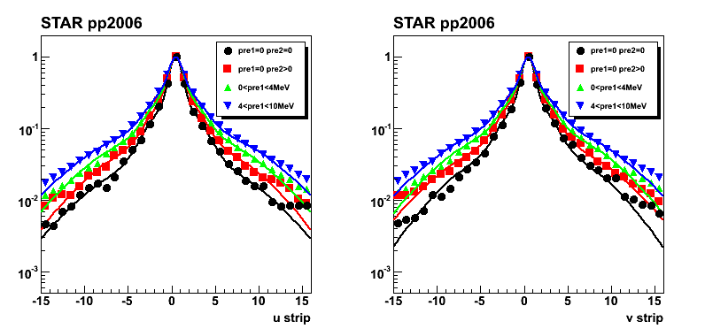
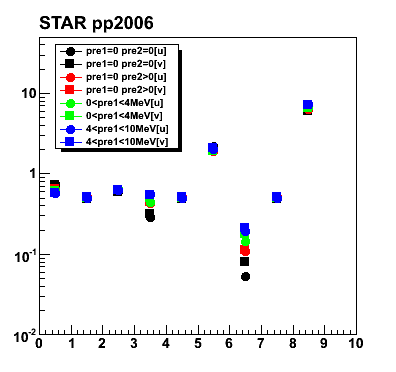
Figure 7: Same as Fig. 5, but for gamma-jet candidates from pp2006 data
2008.09.09 Maximum sided residual with shower shapes sorted by uv- and pre-shower bins
Ilya Selyuzhenkov September 09, 2008
Data sets:
- pp2006 - STAR 2006 pp longitudinal data (~ 3.164 pb^1) after applying gamma-jet isolation cuts.
- gamma-jet - data-driven Pythia gamma-jet sample (~170K events). Partonic pt range 5-35 GeV.
- QCD jets - data-driven Pythia QCD jets sample (~4M events). Partonic pt range 3-65 GeV.
Procedure to calculate maximum sided residual:
-
For each event fit SMD u and v energy distributions with
triple Gaussian functions from shower shapes analysis:[0]*(exp(-0.5*((x-[1])/[2])**2)+[3]*exp(-0.5*((x-[1])/[4])**2)+[6]*exp(-0.5*((x-[1])/[5])**2))
Fit parameters sorted by various pre-shower conditions and u and v-planes can be found here
There are only two free parameters in a final fit: overall amplitude [0] and mean value [1]
Fit range is +-2 strips from the high strip (5 strips total). -
Integrate energy from a fit within +-2 strips from high strip.
This is our peak energy from fit, F_peak. -
Calculate tail energies on left and right sides from the peak for both data, D_tail, and fit, F_tail.
Tails are integrated up to 30 strips excluding 5 highest strips.
Determine maximum difference between D_tail and F_tail:
max(D_tail-F_tail). This is our maximum sided residual. -
Plot F_peak vs. max(D_tail-F_tail). This is sided residual plot.
-
(implementation for this item is in progress)
Based on MC gamma-jet sided residual plot find a line (some polynomial function)
which will serve as a cut to separate signal and background.
Use that cut line to calculate signal to background ratio
and apply it for the real data analysis.
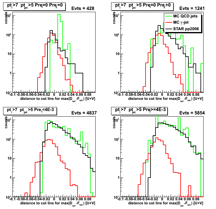
Figure 1: Maximum sided residual plots for different data sets and various pre-shower condition.
Columns [data sets]: 1. MC QCD background; 2. gamma-jet; 3. pp2006 data
Rows [pre-shower bins]: 1. pre1=0 pre2=0; 2. pre1=0, pre2>0; 3. 0<pre1<4MeV; 4. 4<pre1<10MeV
Results from u and v plane are combined as [U+V]/2
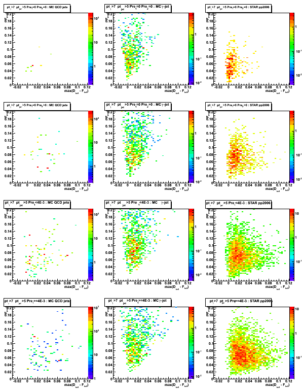
Figure 2: max(D_tail-F_tail) distribution (projection on horizontal axis from Fig.1)
Some observations:
Results for pp2006 and MC gamma-jet are consistent for pre1=0 pre2=0 case (upper left plot)
Results for pp2006 and MC QCD background jets are also in agrees for pre1>0 case (lower left and right plots)
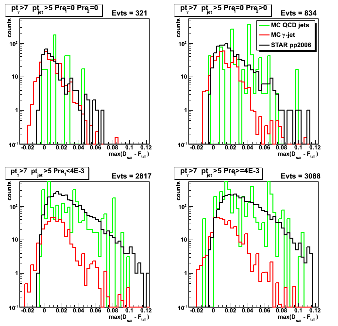
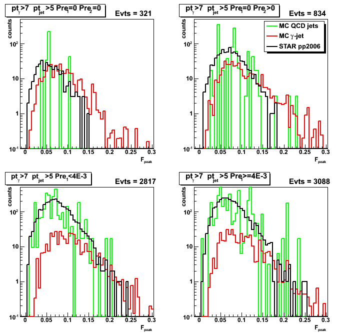
Figure 3: F_peak distribution (projection on vertical axis from Fig.1)
2008.09.16 QA plots for maximum sided residual (obsolete)
Ilya Selyuzhenkov September 16, 2008
These results are obsolete.
Please use this link instead
Data sets:
- pp2006 - STAR 2006 pp longitudinal data (~ 3.164 pb^1) after applying gamma-jet isolation cuts.
- gamma-jet - data-driven Pythia gamma-jet sample (~170K events). Partonic pt range 5-35 GeV.
- QCD jets - data-driven Pythia QCD jets sample (~4M events). Partonic pt range 3-65 GeV.
Notations used in the plots:
- Fit peak energy:
F_peak - integral within +-2 strips from maximum strip
Maximum strip determined by fitting procedure.
Float value converted ("cutted") to integer value. - Data peak energy:
D_peak - energy sum within +-2 strips from maximum strip (the same strip Id as for F_peak). - Data tails:
D_tail^left and D_tail^right.
Energy sum from 3rd strip up to 30 strips on the
left and right sides from maximum strip (excludes strips which contributes to D_peak) - Fit tails:
F_tail^left and F_tail^right.
Same definition as for D_tail, but integrals are calculated from a fit function. - Maximum sided residual:
max(D_tail-F_tail)
Maximum of the data minus fit energy on the left and right sides from the peak.
Figure 1: D_peak from [U+V]/2.
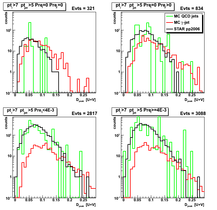
Figure 2: U/V asymmetry for D_peak: [U-V]/[U+V]
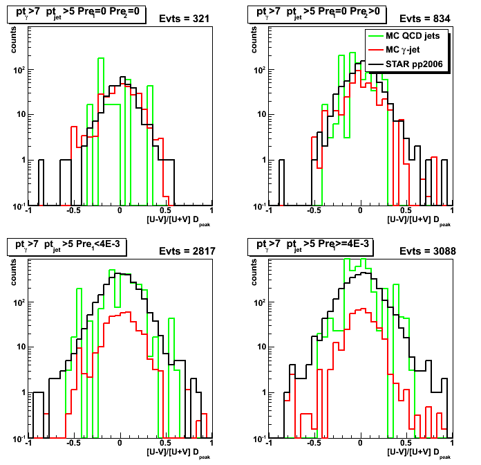
Figure 3: F_peak from [U+V]/2.
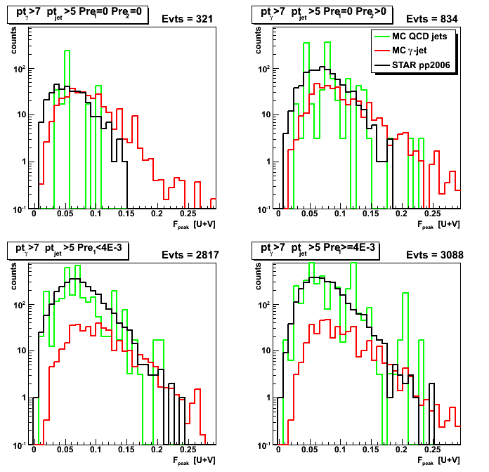
Figure 4: U/V asymmetry for F_peak: [U-V]/[U+V]
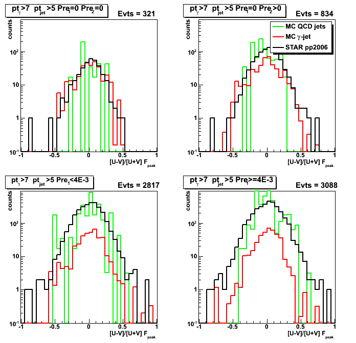
Figure 5: (D_peak - F_peak)/D_peak asymmetry
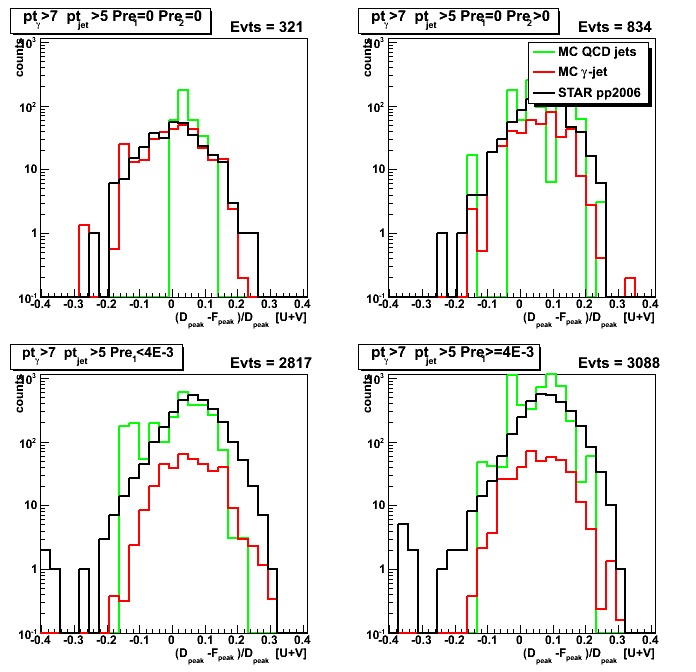
Figure 6: Maximum sided residual from V vs. U plane.
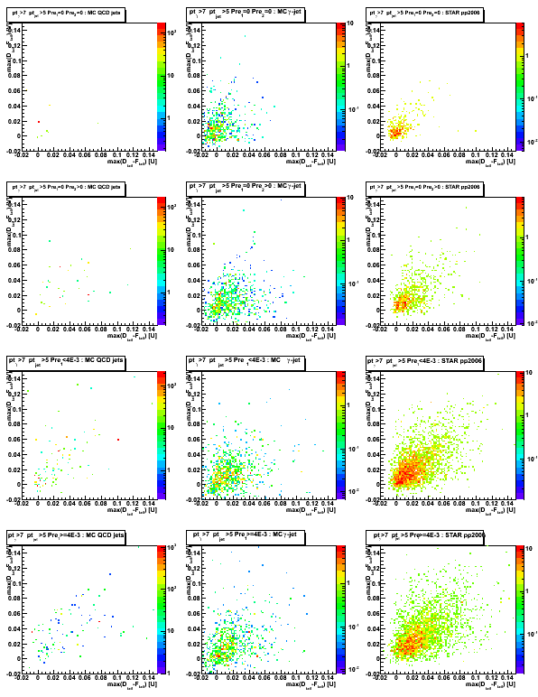
Figure 7: (D_tail-F_tail)^right vs. (D_tail-F_tail)^left
2008.09.23 QA plots for maximum sided residual (bug fixed update)
Ilya Selyuzhenkov September 23, 2008
Data sets:
- pp2006 - STAR 2006 pp longitudinal data (~ 3.164 pb^1)
after applying gamma-jet isolation cuts (note: R_cluster > 0.9 is used below). - gamma-jet - data-driven Pythia gamma-jet sample (~170K events). Partonic pt range 5-35 GeV.
- QCD jets - data-driven Pythia QCD jets sample (~4M events). Partonic pt range 3-65 GeV.
Notations used in the plots:
- Fit peak energy:
F_peak - integral within +-2 strips from maximum strip
Maximum strip determined by fitting procedure.
Float value converted ("cutted") to integer value. - Data peak energy:
D_peak - energy sum within +-2 strips from maximum strip (the same strip Id as for F_peak). - Data tails:
D_tail^left and D_tail^right.
Energy sum from 3rd strip up to 30 strips on the
left and right sides from maximum strip (excludes strips which contributes to D_peak) - Fit tails:
F_tail^left and F_tail^right.
Same definition as for D_tail, but integrals are calculated from a fit function. - Maximum sided residual:
max(D_tail-F_tail)
Maximum of the data minus fit energy on the left and right sides from the peak.
Figure 1: D_peak from [U+V]/2.
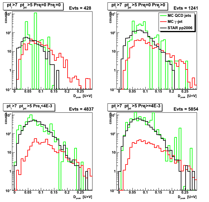
Figure 2: (D_peak - F_peak)/D_peak asymmetry
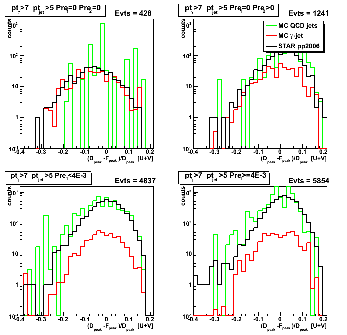
Figure 3: Maximum sided residual from V vs. U plane.
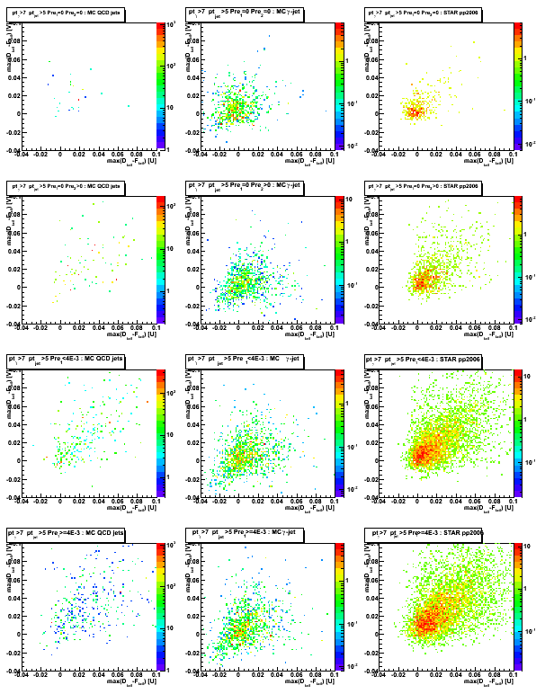
Figure 4: (D_tail-F_tail)^right. (D_tail-F_tail)^left
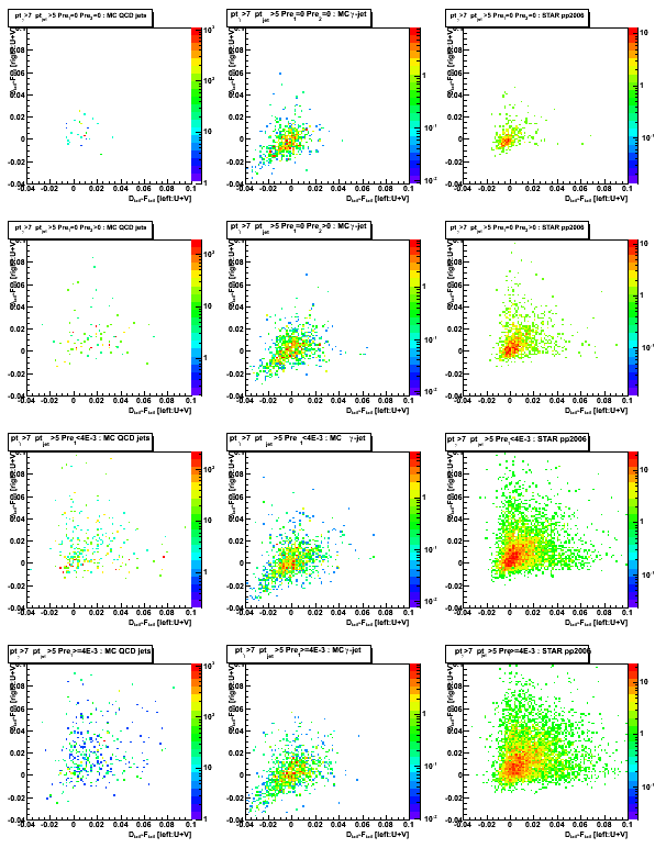
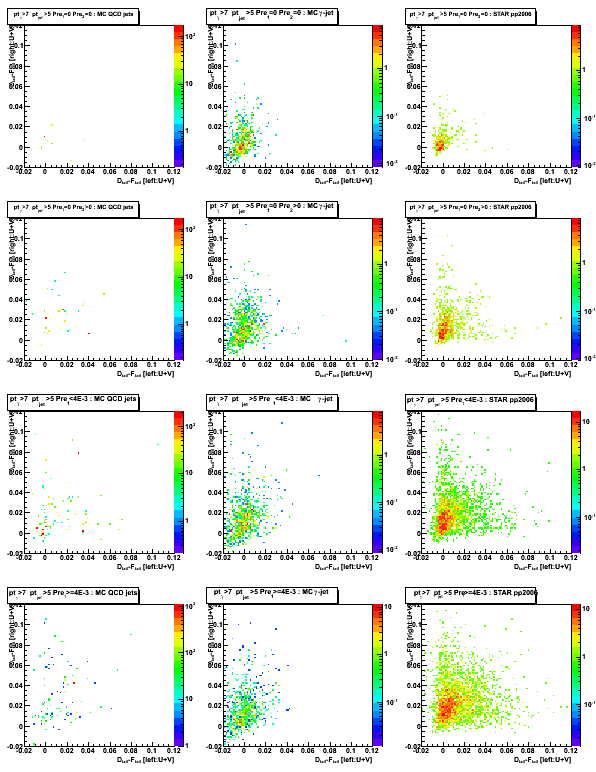
2008.09.23 Right-left SMD tail asymmetries
Ilya Selyuzhenkov September 23, 2008
Figure 1: D_peak vs. [right-left] D_tail
Figure 2: [right-left]/[right-+left] D_tail
2008.09.23 Sided residual plot projection: toward s/b efficency/rejection plot
Ilya Selyuzhenkov September 23, 2008
Data sets:
- pp2006 - STAR 2006 pp longitudinal data (~ 3.164 pb^1)
after applying gamma-jet isolation cuts (note: R_cluster > 0.9 is used below). - gamma-jet - data-driven Pythia gamma-jet sample (~170K events). Partonic pt range 5-35 GeV.
- QCD jets - data-driven Pythia QCD jets sample (~4M events). Partonic pt range 3-65 GeV.
Notations used in the plots:
- Fit peak energy:
F_peak - integral within +-2 strips from maximum strip
Maximum strip determined by fitting procedure.
Float value converted ("cutted") to integer value. - Data peak energy:
D_peak - energy sum within +-2 strips from maximum strip (the same strip Id as for F_peak). - Data tails:
D_tail^left and D_tail^right.
Energy sum from 3rd strip up to 30 strips on the
left and right sides from maximum strip (excludes strips which contributes to D_peak) - Fit tails:
F_tail^left and F_tail^right.
Same definition as for D_tail, but integrals are calculated from a fit function. - Maximum sided residual:
max(D_tail-F_tail)
Maximum of the data minus fit energy on the left and right sides from the peak.
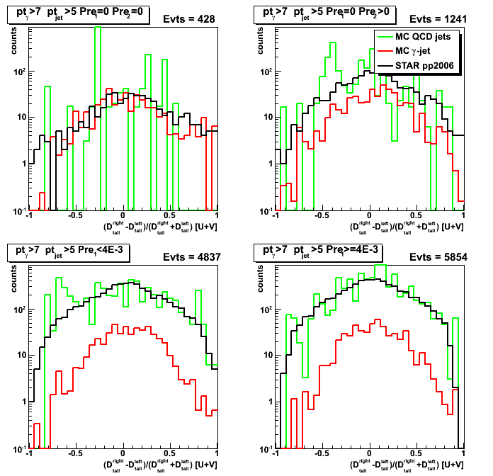
Maximum sided residual: MC vs. data comparison
Figure 1: Maximum sided residual plot
Top get more statistics for MC QCD sample plot is redone with a softer R_cluster > 0.9 cut
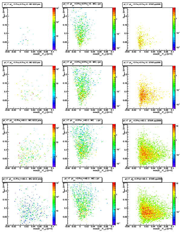
Figure 2: D_peak (projection on vertical axis for Fig. 1)
Upper left plot (no pre-shower fired case) reveals some difference
between MC gamma-jet and pp2006 data at lower D_peak values.
This difference could be due to background contribution at low energies.
Still needs more statistics for MC QCD jet sample to confirm that statement.
Figure 3: max(D_tail-F_tail) (projection on horisontal axis for Fig. 1)
One can get an idea of signal/background separation (red vs. black) depending on pre-shower condition.
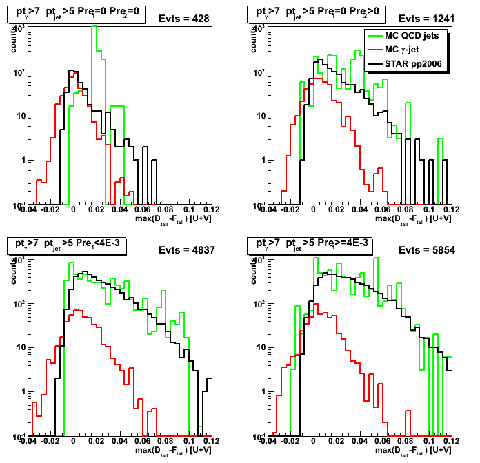
Figure 4: Mean < max(D_tail-F_tail) > vs. D_peak (profile on vertical axis from Fig. 1)
For gamma-jet sample average sided residual is independent on D_peak energy
and has a slight positive shift for all pre-shower>0 conditions.
For large D_peak values (D_peak>0.16) MC gamma-jet and pp2006 data results are getting close to each other.
This corresponds to higher energy gammas, where we have a better signal/background ratio,
and thus more real gammas among gamma-jet candidates from pp2006 data.
(Note: legend's color coding is wrong, colors scheme is the same as in Fig. 3)
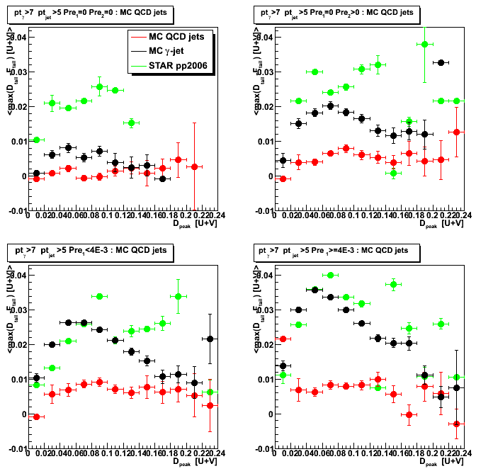
Figure 5: Mean < D_peak > vs. max(D_tail-F_tail) (profile on horisontal axis from Fig. 1)
For "no-preshower fired" case MC gamma-jet sample has a large average values than that from pp2006 data.
This reflects the same difference between pp2006 and MC gamma-jet sample at small D_peak values (see Fig. 2, upper left plot).
(Note: legend's color coding is wrong, colors scheme is the same as in Fig. 3)
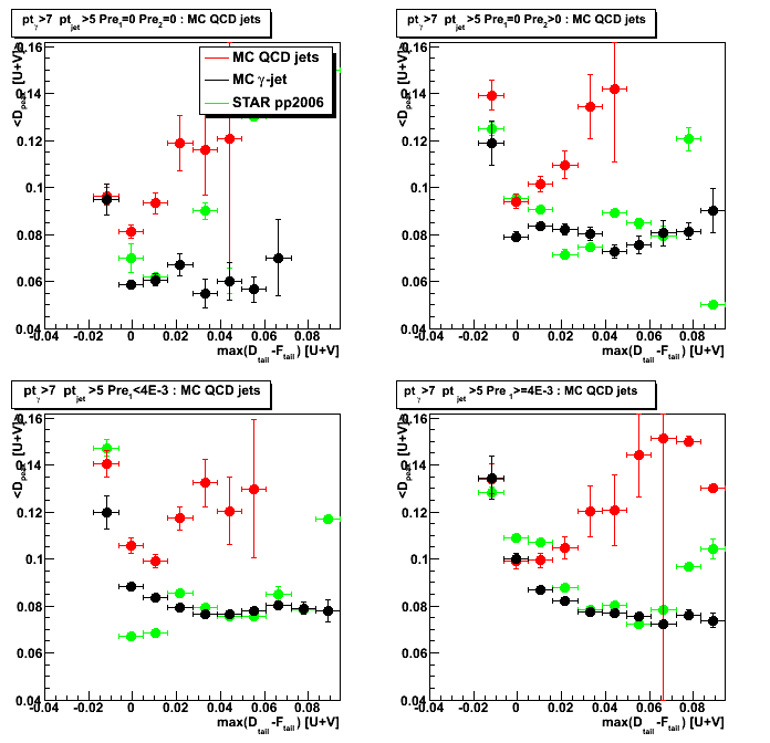
Figure 6: D_peak vs. gamma pt
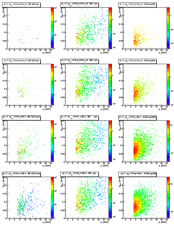
Figure 7: D_peak vs. gamma 3x3 tower cluster energy
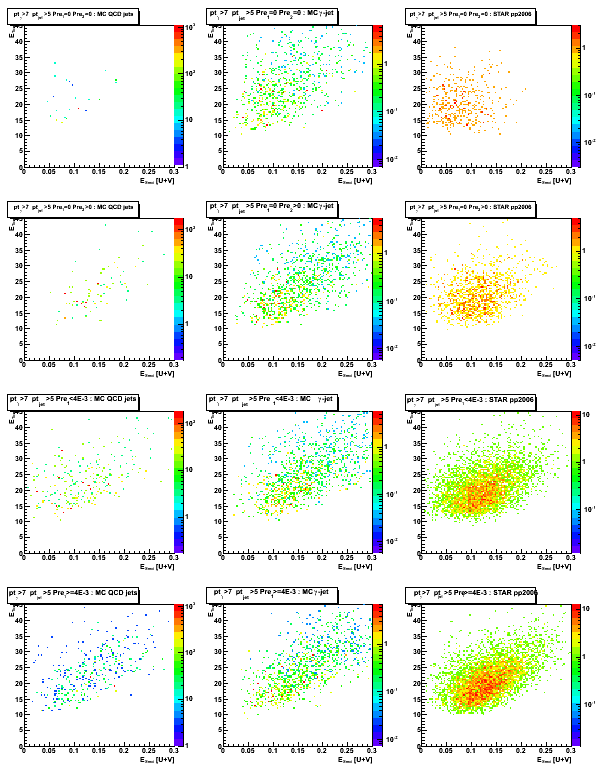
Figure 8: 3x3 cluster tower energy distribution
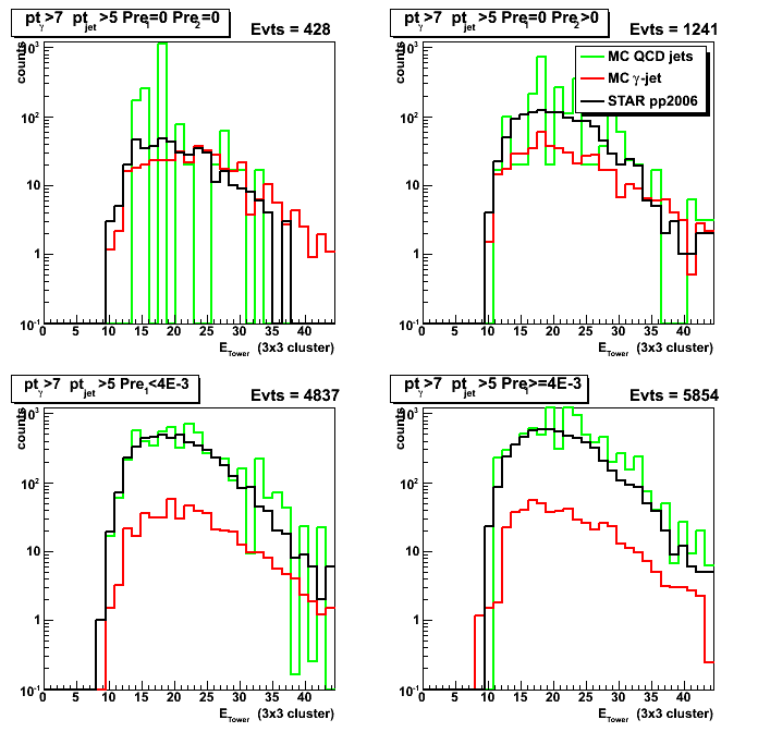
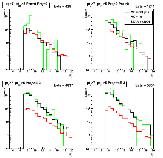
Figure 9: Gamma pt distribution
Signal/background separation
The simplest way to get signal/background separation is to draw a straight line
on sided residual plot (Fig. 1) in such a way that
it will contains most of the counts (signal) on the left side,
and use a distance to that line for both MC and pp2006 data samples
as a discriminant for signal/background separation.
To get the distance to the straight line one can rotate sided residual plot
by the angle which corresponds to the slope of this line,
and then project it on "rotated" max(D_tail-F_tail) axis.
Figure 10: Shows "rotated" sided residual plot by "5/6*(pi/2)" angle (this angle has been picked by eye).
One can see that now most of the counts for gamma-jet sample (middle column)
are on the left side from vertical axis.
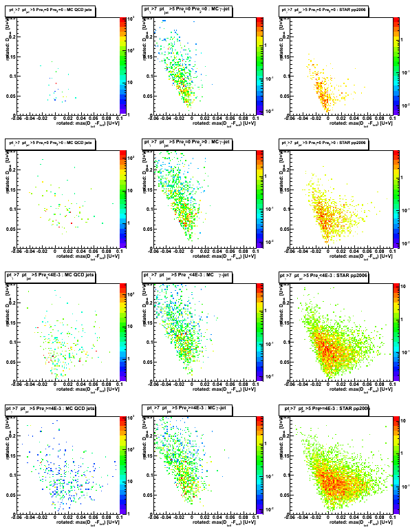
Figure 11: "Rotated" max(D_tail-F_tail) [projection on horizontal axis for Fig. 10]
Cut on "Rotated" max(D_tail-F_tail) can be used for signal/background separation.
From figure below one can see much better signal/background separation than in Fig. 3
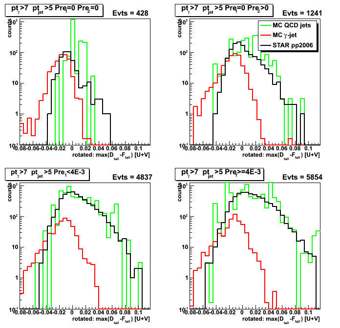
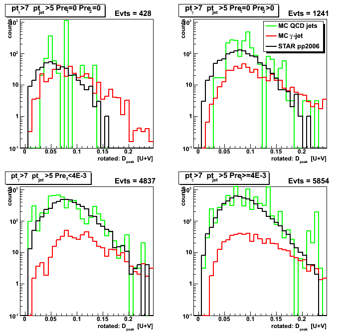
Figure 12: "Rotated" D_peak [projection on vertical axis for Fig. 10]
Optimizing the shape of s/bg separation line
Ideally, instead of straight line one needs to use
an actual shape of side residual distribution for MC gamma-jet sample.
This shape can be extracted and parametrized by the following procedure:
- Get slices from sided residual plot for different D_peak values
- From each slice get max(D_tail-F_tail) value
for which most of the counts appears on its left side (for example 80%), - Fit these set of points {D_peak slice, max(D_tail-F_tail)} with a polynomial function
The distance to that polynomial function can be used to determine our signal/background rejection efficiency.
This work is in progress...
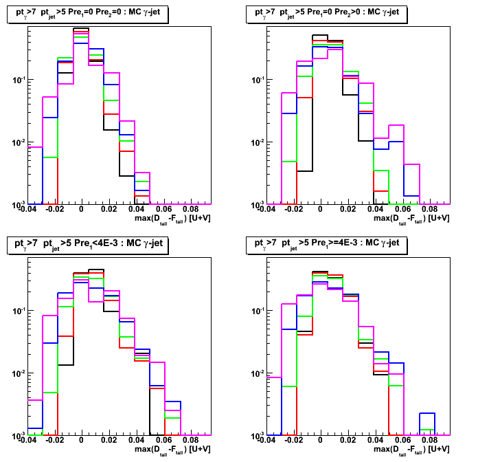
Just last one figure showing shapes for 6 slices from sided plot.
Figure 13: max(D_tail-F_tail) for different slices in D_peak (scaled by the integral for each slice)
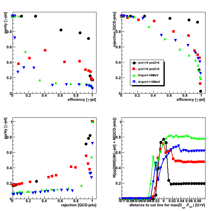
2008.09.30 Sided residual: purity, efficiency, and background rejection
Ilya Selyuzhenkov September 30, 2008
Data sets:
- pp2006 - STAR 2006 pp longitudinal data (~ 3.164 pb^1)
after applying gamma-jet isolation cuts (note: R_cluster > 0.9 is used below). - gamma-jet - data-driven Pythia gamma-jet sample (~170K events). Partonic pt range 5-35 GeV.
- QCD jets - data-driven Pythia QCD jets sample (~4M events). Partonic pt range 3-65 GeV.
Notations used in the plots:
- Fit peak energy:
F_peak - integral within +-2 strips from maximum strip
Maximum strip determined by fitting procedure.
Float value converted ("cutted") to integer value. - Data peak energy:
D_peak - energy sum within +-2 strips from maximum strip (the same strip Id as for F_peak). - Data tails:
D_tail^left and D_tail^right.
Energy sum from 3rd strip up to 30 strips on the
left and right sides from maximum strip (excludes strips which contributes to D_peak) - Fit tails:
F_tail^left and F_tail^right.
Same definition as for D_tail, but integrals are calculated from a fit function. - Maximum sided residual:
max(D_tail-F_tail)
Maximum of the data minus fit energy on the left and right sides from the peak.
Determining cut line based on sided residual plot
Figure 1: Sided residual plot: D_peak vs. max(D_tail-F_tail)
Red lines show 4th order polynomial functions, a*x^4,
which have 80% of MC gamma-jet counts on the left side.
These lines are obtained independently for each of pre-shower condition
based on fit procedure shown in Fig. 3 below.
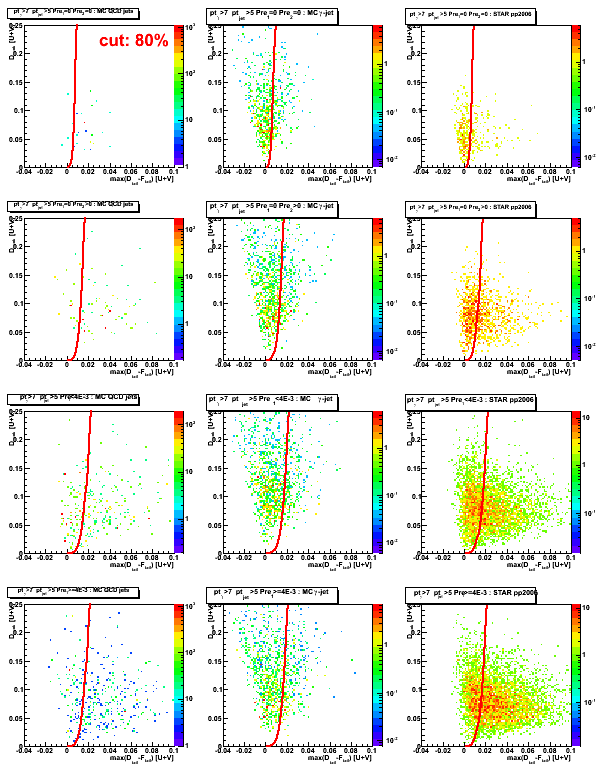
Figure 2: max(D_tail-F_tail) distribution
(projection on horizontal axis from sided residual plot, see Fig. 1 above)
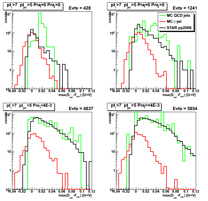
Figure 3: max(D_tail-F_tail) [at 80%] vs. D_peak.
For each slice (bin) in D_peak variable, the max(D_tail-F_tail) value
which has 80% of gamma-jet candidates on the left side are plotted.
Lines represent fits to MC gamma-jet points (shown in red) using different fit functions
(linear, 2nd, 4th order polynomials: see legend for color coding).
Note, that in this plot D_peak values are shown on horizontal axis.
Consequently, to get 2nd order polynomial fit on sided residual plot (Fig. 1),
one needs to use sqrt(D_peak) function.
The same apply to 4th order polynomial function.
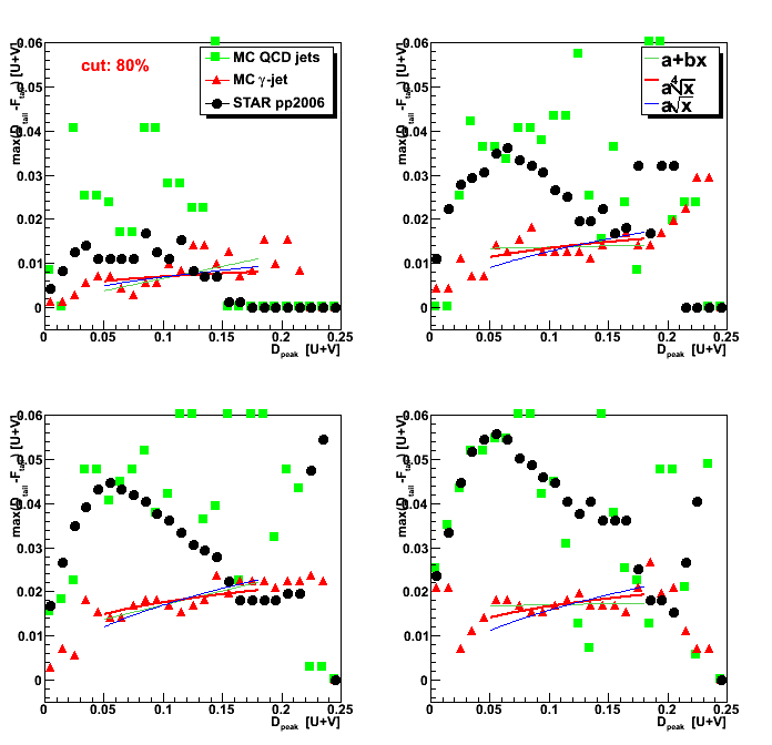
Figure 4: D_peak vs. horisontal distance from 4th order polinomial function to max(D_tail-F_tail) values.
(compare with Fig. 1: Now 80% of MC gamma-jet counts are on the left side from vertical axis)
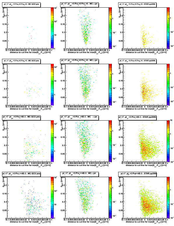
Figure 5: Horizontal distance from 4th order polynomial function to max(D_tail-F_tail)
[Projection on horizontal axis from Fig. 4]
Based on this plot one can obtain purity, efficiency, and rejection plots (see Fig. 6 below)
Gamma-jet purity, efficiency, and QCD background rejection
Horizontal distance plotted in Fig. 5 can be used as a cut
separating gamma-jet signal and QCD-jets background,
and for each value of this distance one can define
gamma-jet purity, efficiency, and QCD-background rejection:
-
gamma-jet purity is defined as the ratio of
the integral on the left for MC gamma-jet data sample, N[g-jet]_left,
to the sum of the integrals on the left for MC gamma-jet and QCD jets, N[QCD]_left, data samples:
Purity[gamma-jet] = N[g-jet]_left/(N[g-jet]_left+N[QCD]_left) -
gamma-jet efficiency is defined as the ratio of
the integral on the left side for MC gamma-jet data sample, N[g-jet]_left,
to the total integral for MC gamma-jet data sample, N[g-jet]:
Efficiency[gamma-jet] = N[g-jet]_left/N[g-jet] -
QCD background rejection is defined as the ratio of
the integral on the right side for MC QCD jets data sample, N[QCD]_right,
to the total integral for MC QCD jets data sample, N[QCD]:
Rejection[QCD] = N[QCD]_right/N[QCD]
Figure 6: Shows:
purity[g-jet] vs. efficiency[g-jet] (upper left);
rejection[QCD] vs. efficiency[g-jet] (upper right);
purity[g-jet] vs. rejection[QCD] (lower left);
pp2006 to MC ratio, N[pp2006]/(N[g-jet]+N[QCD]), vs. horizontal distance from Fig. 5 (lower right)