2009.03.02 Application of the neural network for the cut optimization (zero try)

Multilayer perceptron (feedforward neural networks)

Multilayer perceptron (MLP) is feedforward neural networks
trained with the standard backpropagation algorithm.
They are supervised networks so they require a desired response to be trained.
They learn how to transform input data into a desired response,
so they are widely used for pattern classification.
With one or two hidden layers, they can approximate virtually any input-output map.
They have been shown to approximate the performance of optimal statistical classifiers in difficult problems.

ROOT implementation for Multilayer perceptron

TMultiLayerPerceptron class in ROOT
mlpHiggs.C example

Application for cuts optimization in the gamma-jet analysis

Netwrok structure:
r3x3, (pt_gamma-pt_jet)/pt_gamma, nCharge, bBtow, eTow2x1: 10 hidden layers: one output later

Figure 1:

• Upper left: Learning curve (error vs. number of training)
  Learing method is: Steepest descent with fixed step size (batch learning)
• Upper right: Differences (how important are initial variableles for signal/background separation)
• Lower left: Network structure (ling thinkness corresponds to relative weight value)
• Lower right: Network output. Red - MC gamma-jets, blue QCD background, black pp2006 data

 

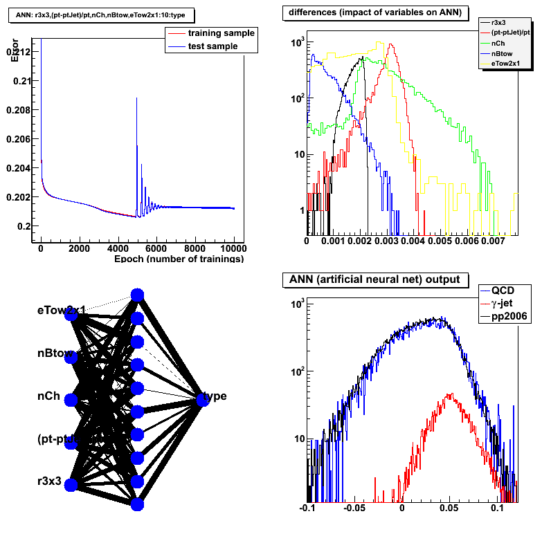
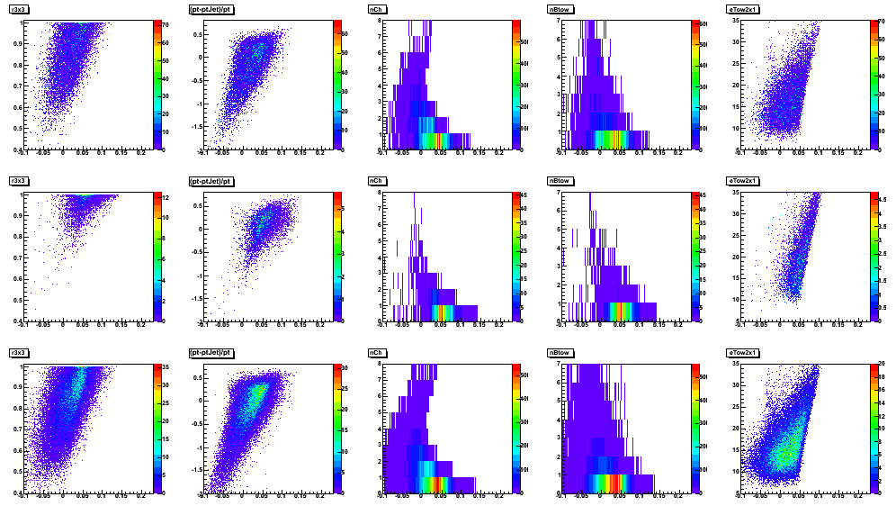
Figure 2: Input parameters vs. network output
Row: 1: MC QCD, 2: gamma-jet, 3 pp2006 data
Vertical axis: r3x3, (pt_gamma-pt_jet)/pt_gamma, nCharge, bBtow, eTow2x1
Horisontal axis: network output

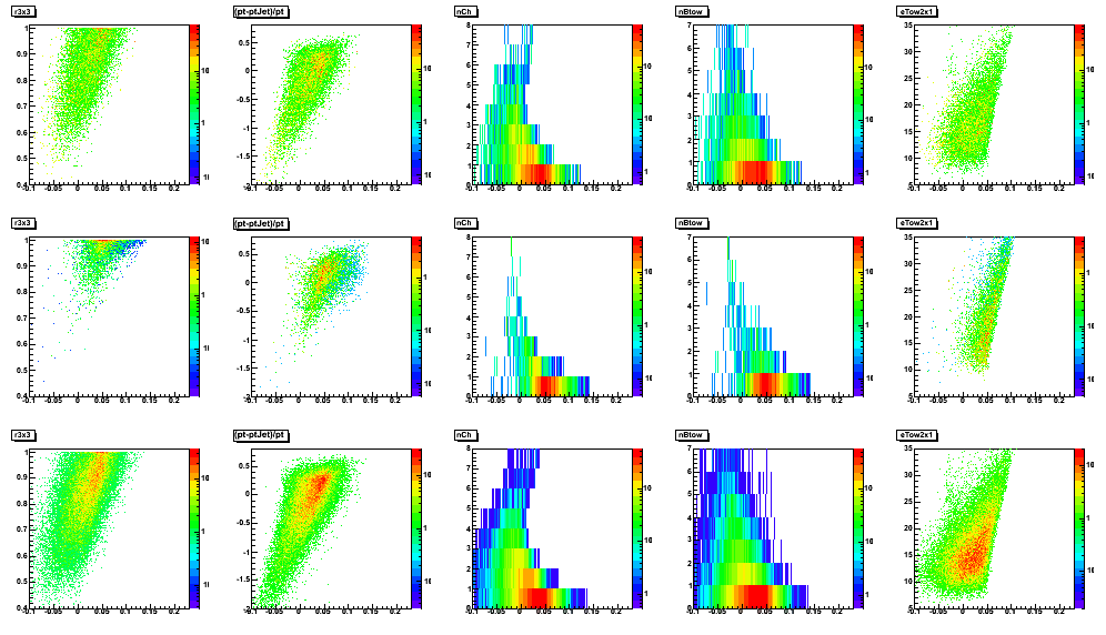
Figure 3: Same as Fig. 2 on a linear scale

2009.03.09 Application of the LDA and MLP classifiers for the cut optimization

Cut optimization with Fisher's LDA and MLP (neural network) classifiers

ROOT implementation for LDA and MLP:

• Fisher's Linear Discriminant Analysis (LDA)
• Multi-Layer Perceptron (MLP) [feed-forward neural network]

Application for cuts optimization in the gamma-jet analysis

LDA configuration: default

MLP configuration:

• 2 hidden layers [N+1:N neural network configuration, N is number of input parameters]
• Learning method: stochastic minimization (1000 learning cycles)

Input parameters (same for both LDA and MLP):

1. Energy fraction in 3x3 cluster within a r=0.7 radius: r3x3
2. Photon-jet pt balance: [pt_gamma-pt_jet]/pt_gamma
3. Number of charge tracks within r=0.7 around gamma candidate
4. Number of Endcap towers fired within r=0.7 around gamma candidate
5. Number of Barrel towers fired within r=0.7 around gamma candidate

Figure 1: Signal efficiency and purity, background rejection (left),
and significance: Sig/sqrt[Sig+Bg] (right) vs. LDA (upper plots) and MLP (lower plots) classifier discriminants

Figure 2:

1. Upper left: Rejection vs. efficiency
2. Upper right: Purity vs. efficiency
3. Lower left: Purity vs. Rejection
4. Lower right: Significance vs. efficiency

 

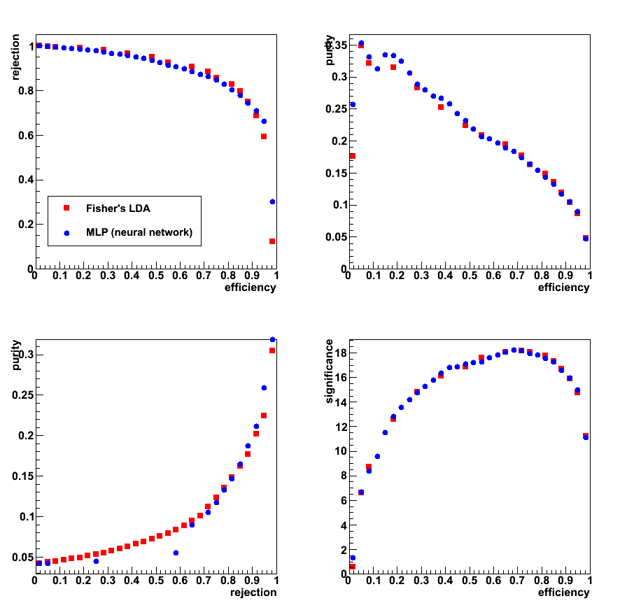
Figure 3: Data to Monte-Carlo comparison for LDA (upper plots) and MLP (lower plots)
Good (within ~ 10%) match between data nad Monte-Carlo
a) up to 0.8 for LDA discriminant, and b) up to -0.7 for MLP.

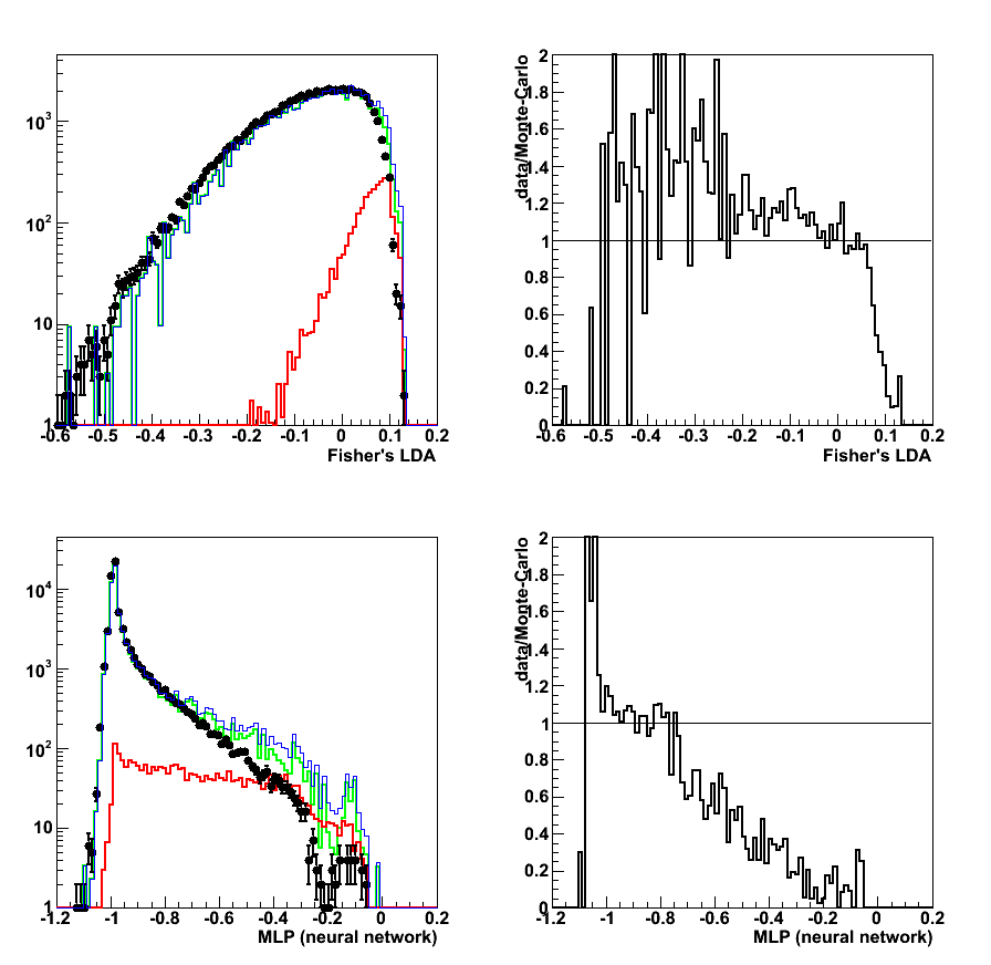
Figure 4: Data to Monte-Carlo comparison for input parameters
from left to right
1) pt_gamma 2) pt_jet 3) r3x3 4) gamma-jet pt balance 5) N_ch[gamma] 6) N_eTow[gamma] 7) N_bTow[gamma]
Colour coding: black pp2006 data, red gamma-jet MC, green QCD MC, blue gamma-jet+QCD

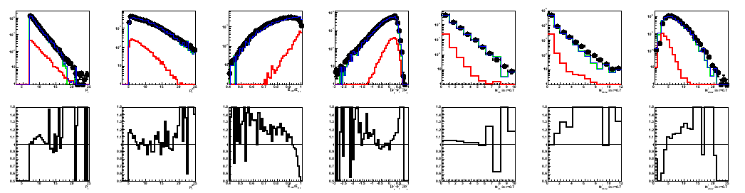
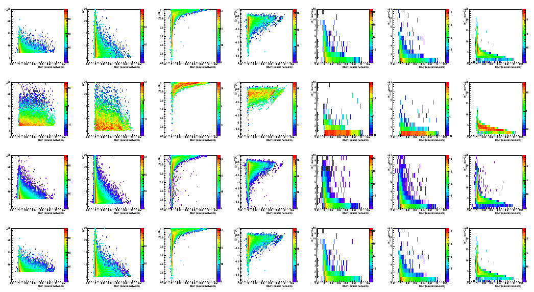
Figure 5: Data to Monte-Carlo comparison:
correlations between input variables (in the same order as in Fig. 4)
and LDA classifier discriminant (horizontal axis).
1st raw: QCD MC; 2nd: gamma-jet MC; 3rd: pp2006 data; 4th: QCD+gamma-jet MC

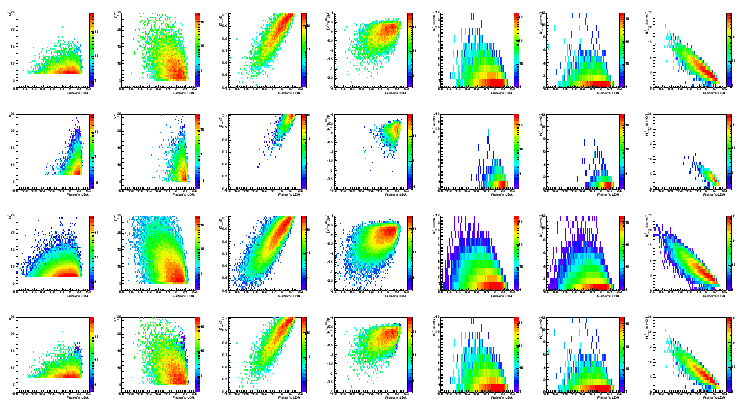
Figure 6: Same as Fig. 6 for MLP discriminant

2009.03.26 Endcap photon-jet update at the STAR Collaboration meeting

Endcap photon-jet update at the STAR Collaboration meeting