2006.07.31 First Look at SMD gamma/pi0 Discrimination

Pibero Djawotho

Indiana University
July 31, 2006

Simulation

Simulation were done by Jason for the SVT review.

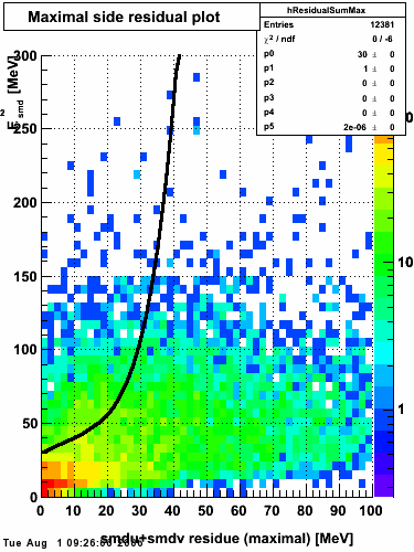
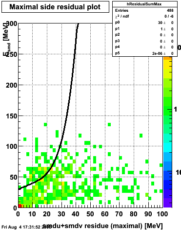
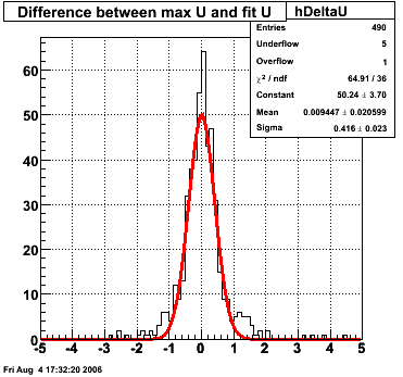
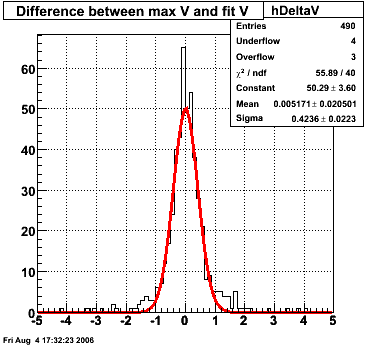
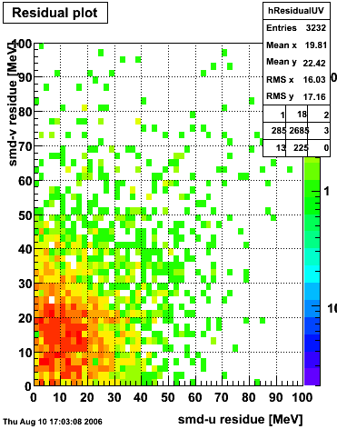
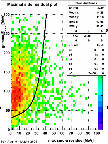
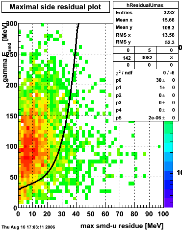
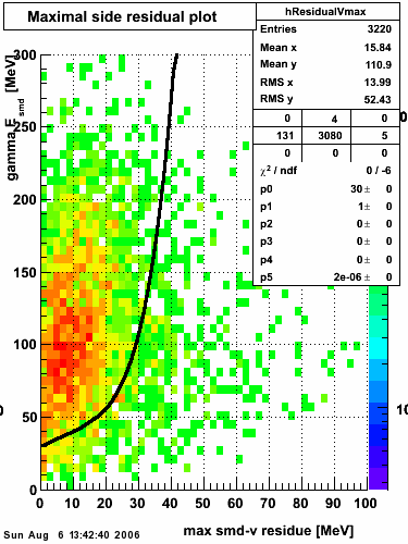
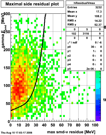
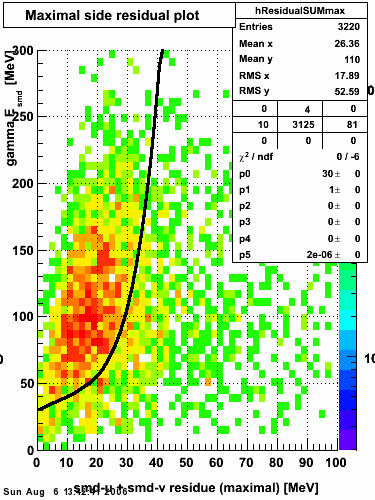
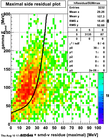
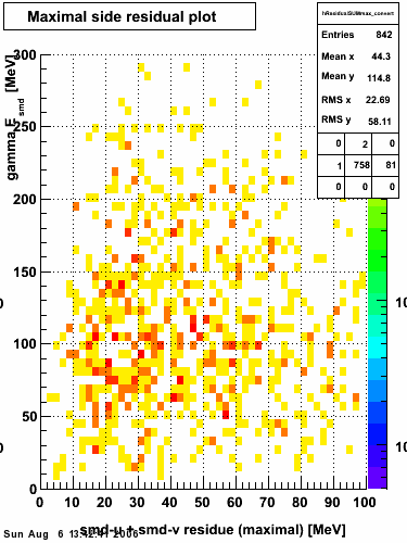
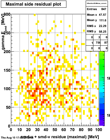
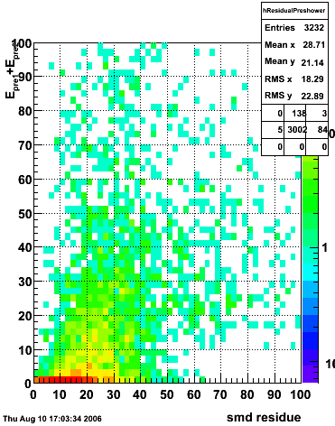
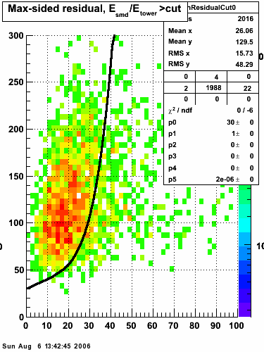
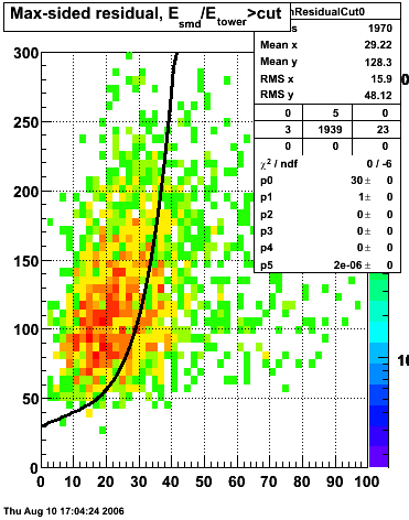
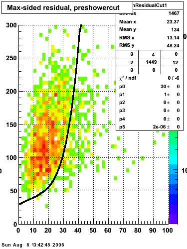
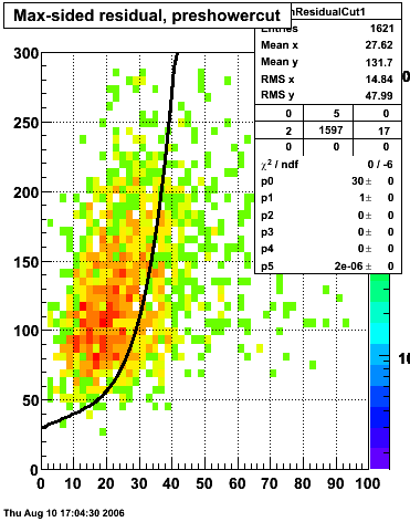
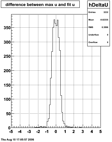
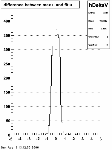
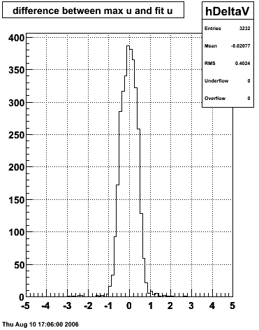
Maximal side residual


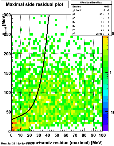Figure 1: Fitted peak integral vs. fit residual sum (U+V) from st_jpsi input stream (J/psi trigger only).	Figure 2: Fitted peak integral vs. fit residual sum (U+V) from st_physics input stream (all triggers except express stream triggers).

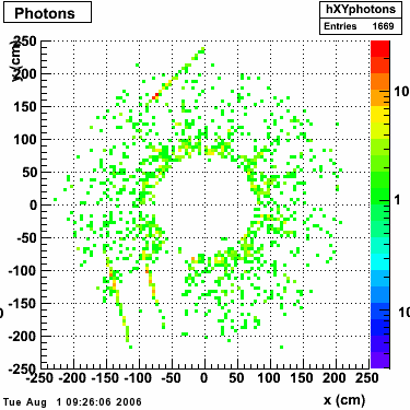
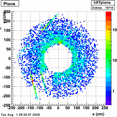
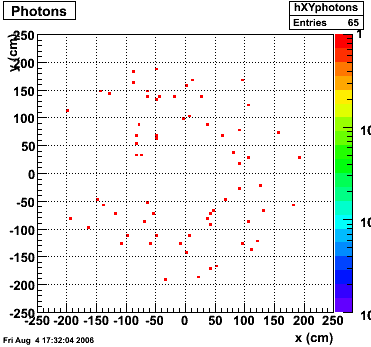
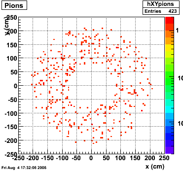
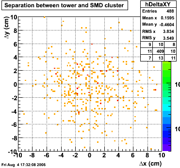
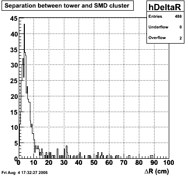
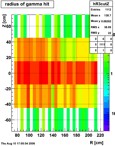
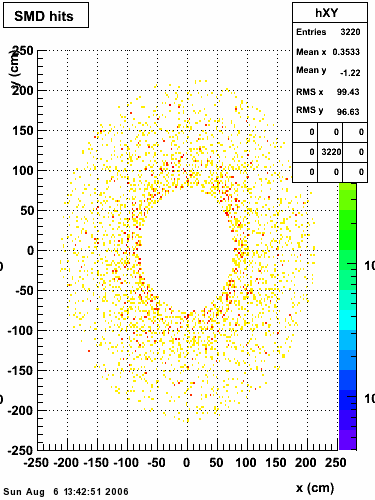
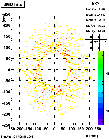
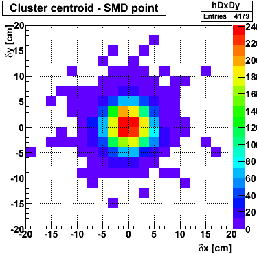
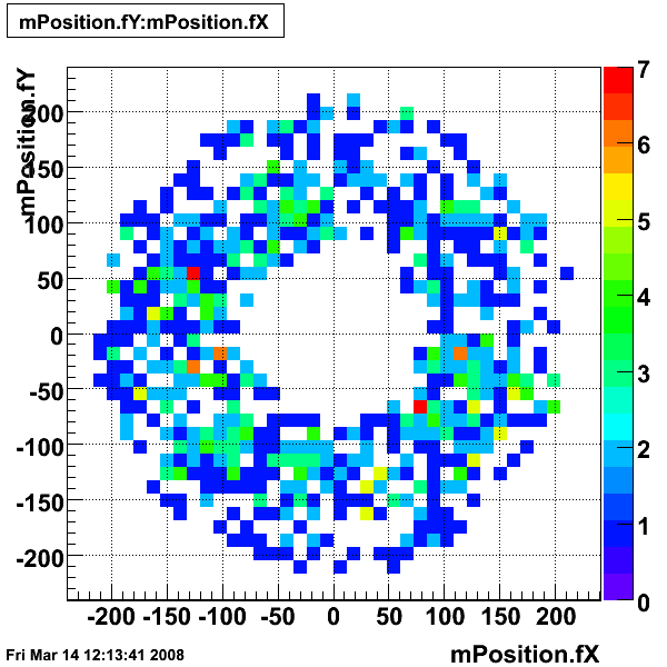
xy distribution of SMD hits

The separation between photons and pions was achieved by using Les cut in the above figures where photons reside above the curve and pions below. The data set used is the st_jpsi express stream.

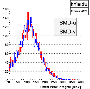
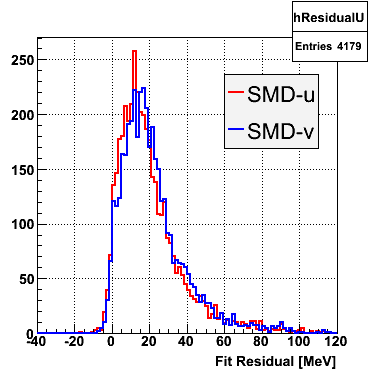
Single peak characteristics

Fit function

The transverse profile of an electromagnetic shower in the SMD can be parametrized by the equation below in each SMD plane:

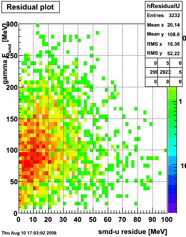
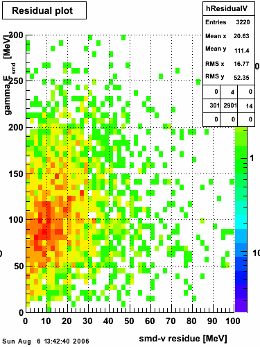
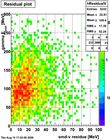
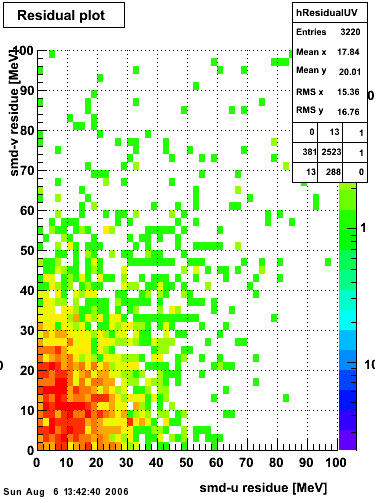
f(x) is the energy in MeV as a function of SMD strip x. The algorithm performs a simultaneous fit in both the U and V plane. The maximal residual (data - fit) is then calculated. A single photon in the SMD should be well descibed by the equation above and therefore will have a smaller maximal residual. A neutral pion, which decays into two photons, should exhibit a larger maximal residual. Typically, the response would be a double peak, possibly a larger peak and a smaller peak corresponding to a softer photon.

Single event SMD response

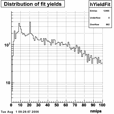
This directory contains images of single event SMD responses in both U and V plane. The file name convention is SMD_RUN_EVENT.png. The fit function for a single peak is the one described in the section above with 5 parameters:

p0 = yield (P₀), area under the peak in MeV
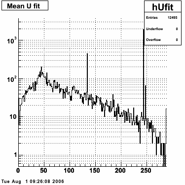
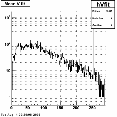
p1 = mean (μ), center of peak in strips
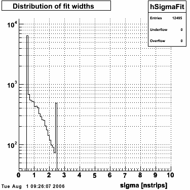
p2 = sigma of the first Gaussian (w₁)
p3 = fraction of the amplitude of the second Gaussian with respect to the first one (B), fixed to 0.2
p4 = ratio of the width of the second Gaussian to the width of the first one (w₂/w₁), fixed to 3.5

Code

macros

Documents

2006.08.04 Second Look at SMD gamma/pi0 Discrimination

Second Look at SMD gamma/pi0 Discrimination

Pibero Djawotho
Indiana University
August 4, 2006

Dataset

The dataset used in this analysis is the 2005 p+p collision at √s=200 GeV with the endcap calorimeter high-tower-1 (eemc-ht1-mb = 96251) and high-tower-2 (eemc-ht2-mb = 96261) triggers.

The file catalog query used to locate the relevant files is:
get_file_list.pl -keys 'path,filename' -delim / -cond 'production=P05if, trgsetupname=ppProduction,filetype=daq_reco_MuDst,filename~st_physics, tpc=1,eemc=1,sanity=1' -delim 0

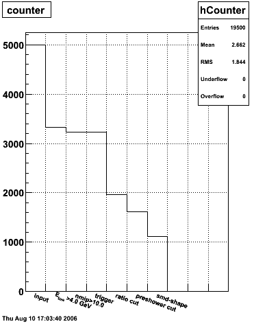
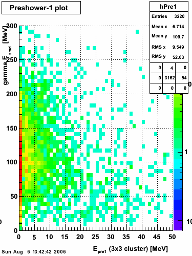
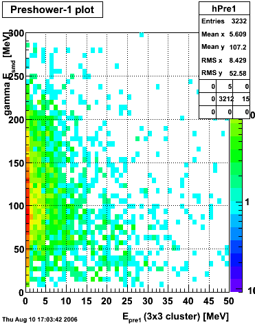
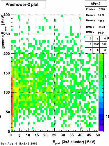
Results

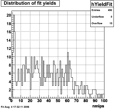
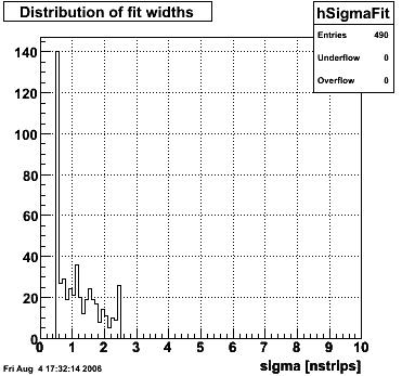
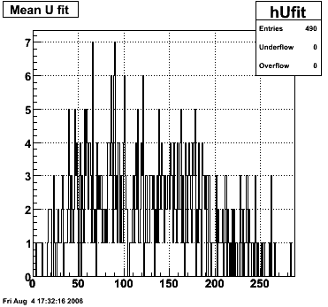
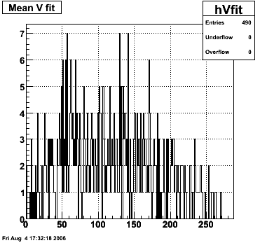
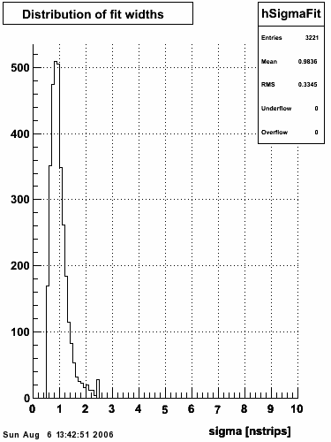
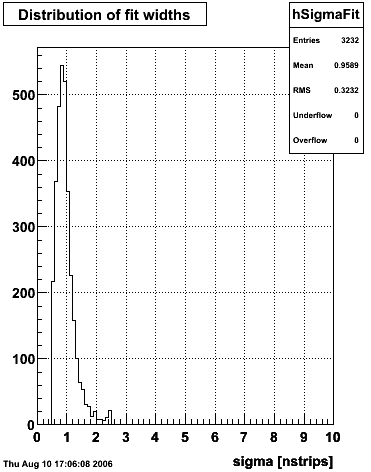
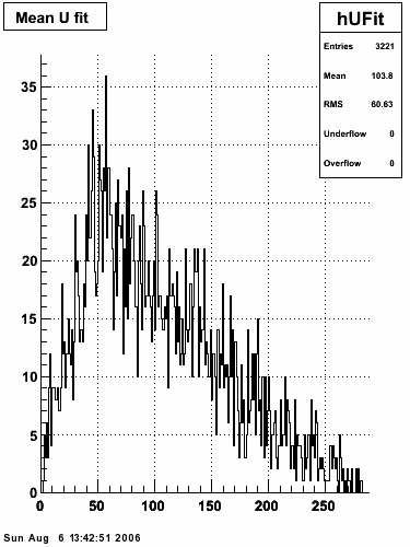
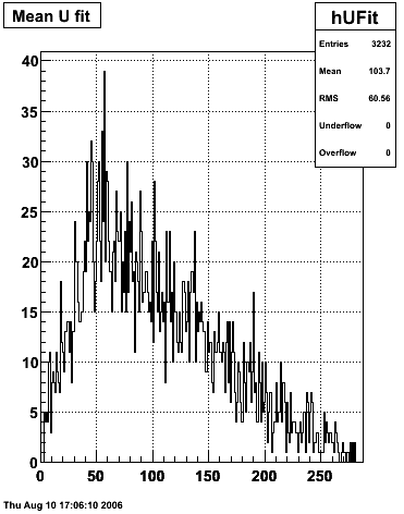
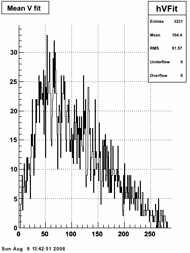
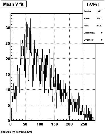
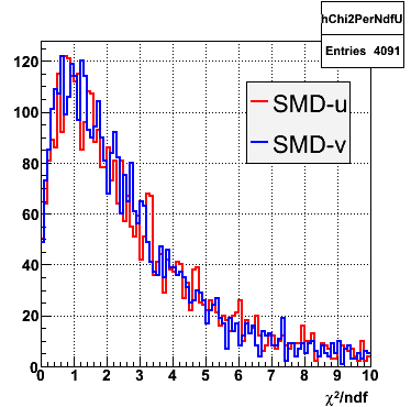
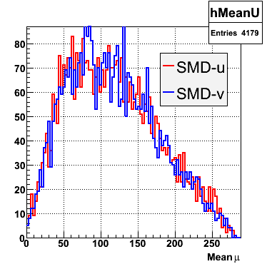
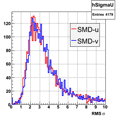
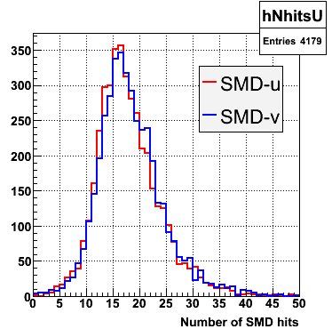
SMD U and V Fits

Code

macros

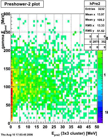
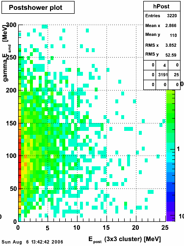
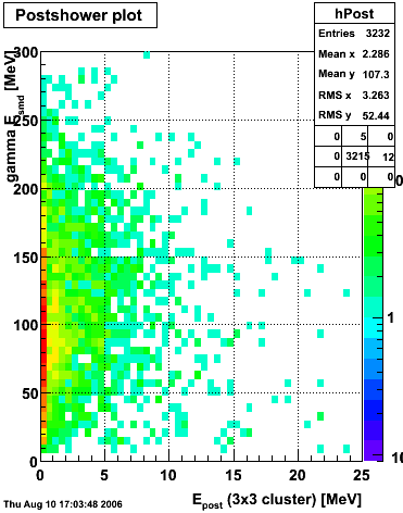
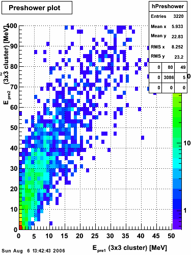
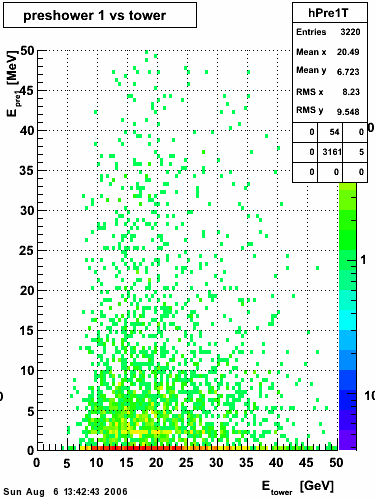
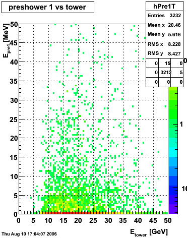
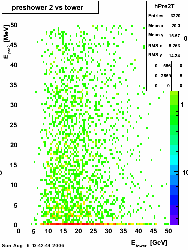
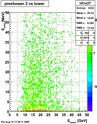
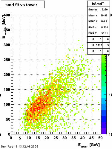
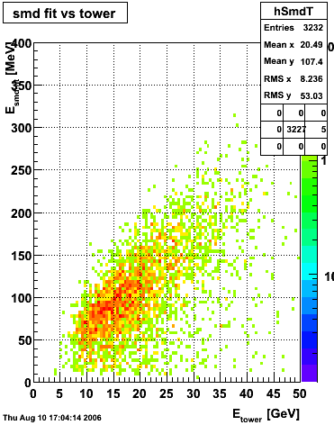
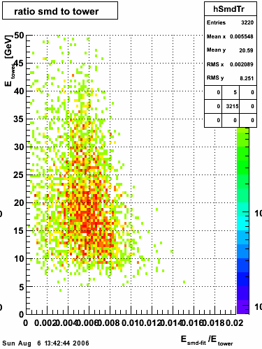
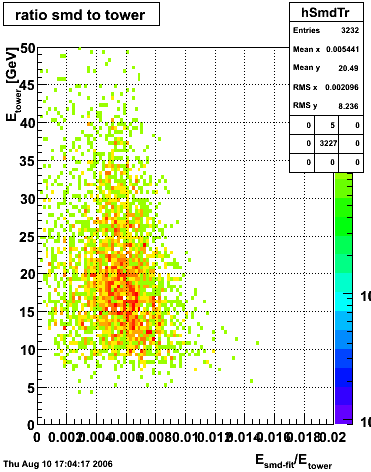
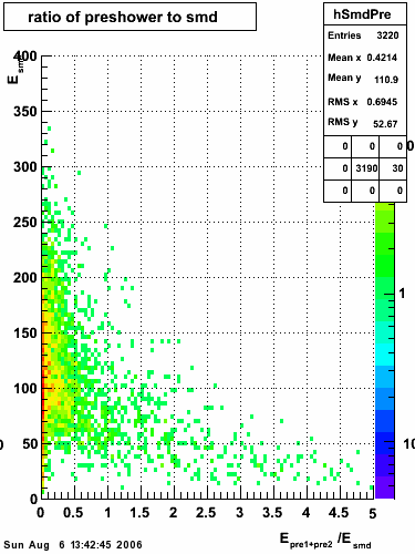
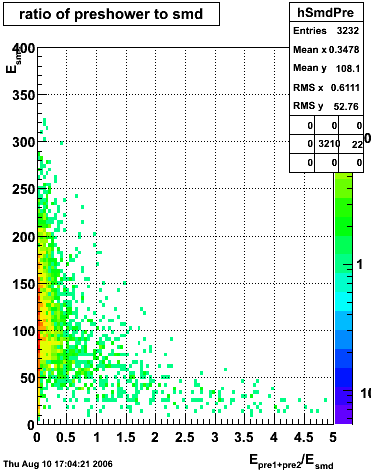
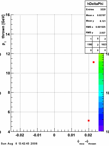
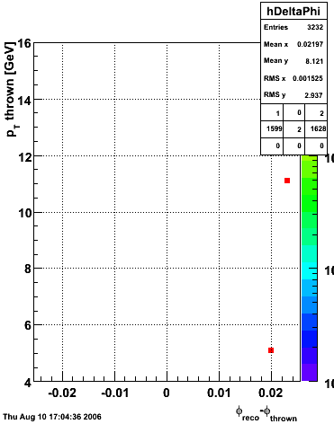
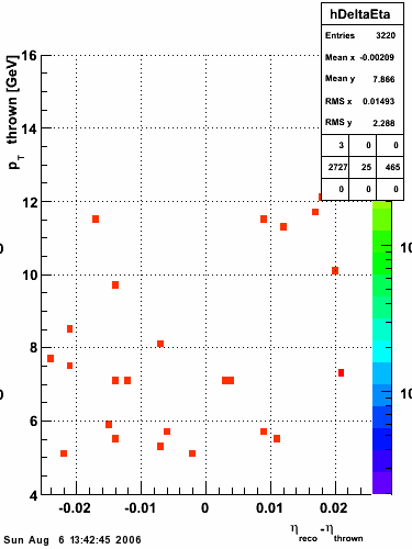
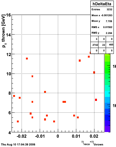
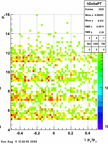
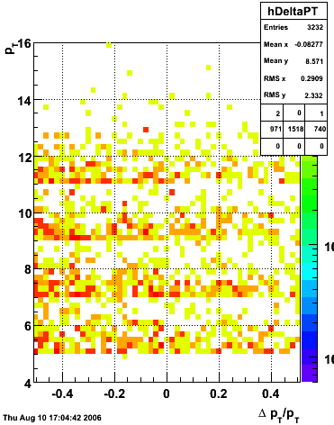
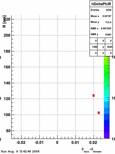
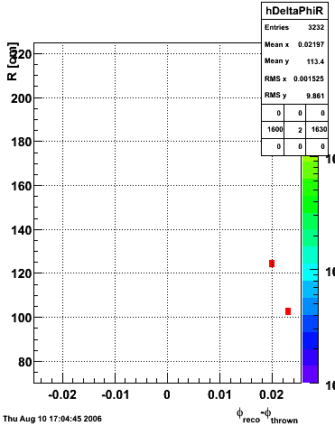
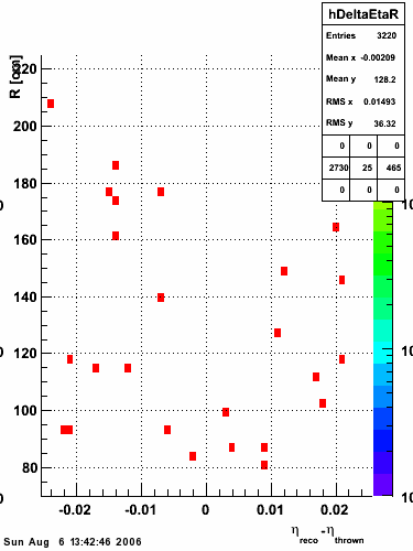
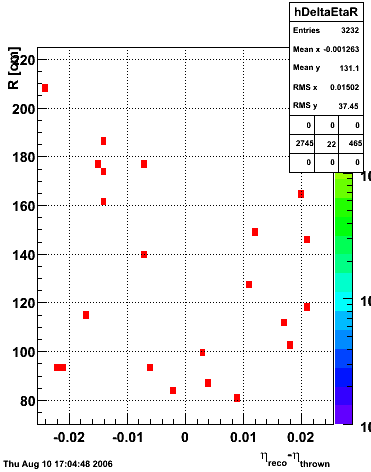
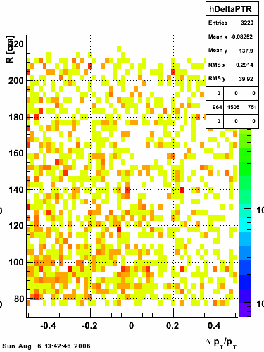
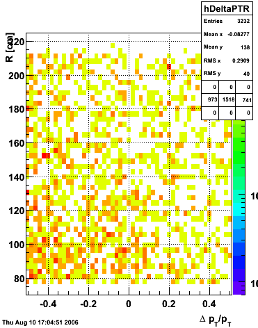
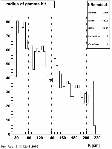
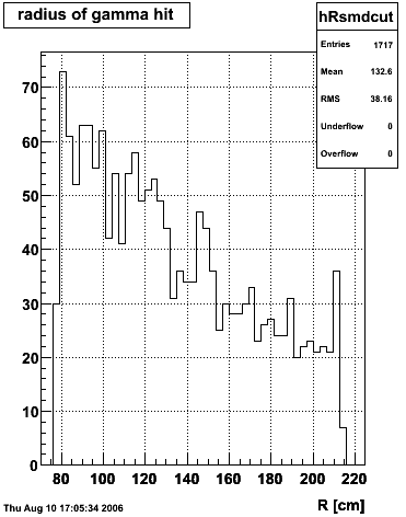
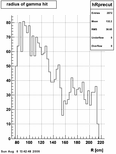
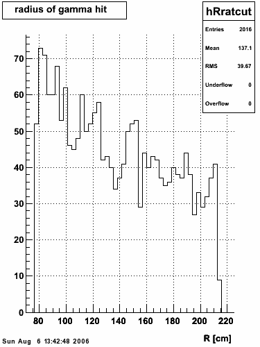
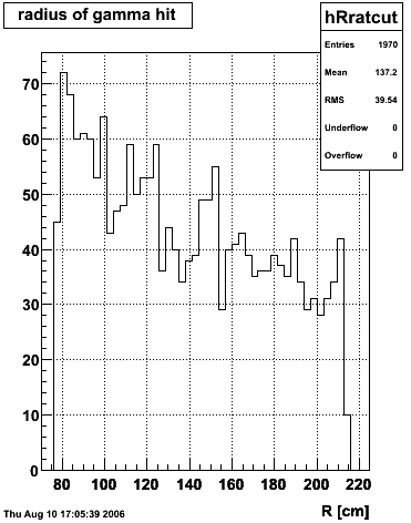
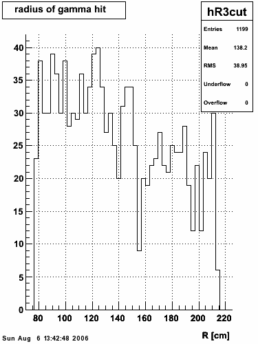
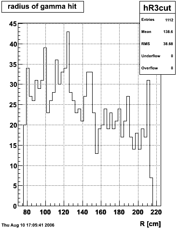
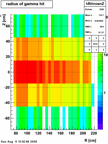
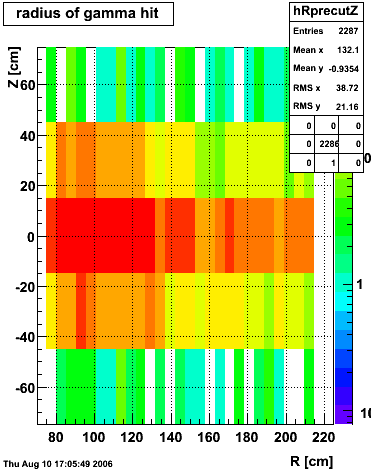
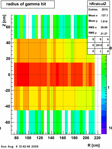
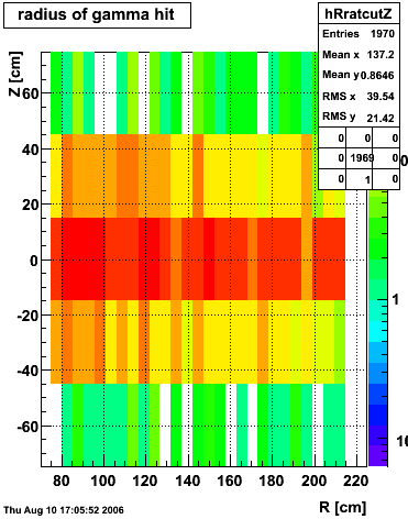
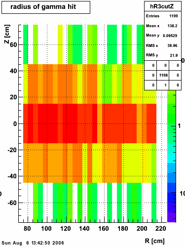
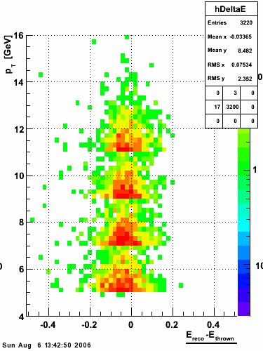
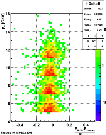
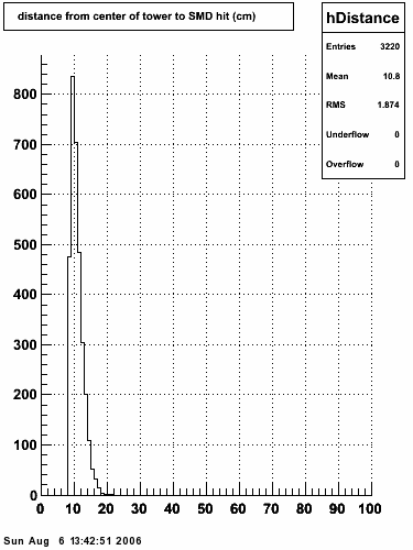
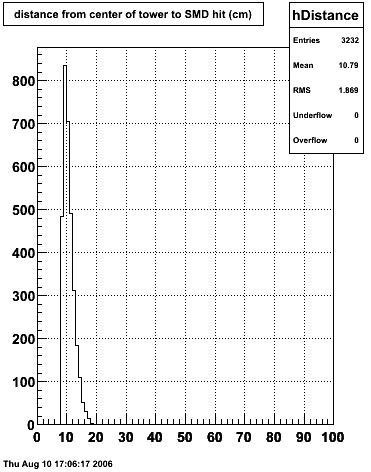
2006.08.06 Comparison between EEMC fast and slow simulator

Comparison between EEMC fast and slow simulator

Pibero Djawotho
Indiana University
August 6, 2006

A detailed description of the EEMC slow simulator is presented at the STAR EEMC Web site.

The following settings were used in running the slow simulator:

  //--
  //-- Initialize slow simulator
  //--
  StEEmcSlowMaker *slowSim = new StEEmcSlowMaker("slowSim");
  slowSim->setDropBad(1);   // 0=no action, 1=drop chn marked bad in db
  slowSim->setAddPed(1);    // 0=no action, 1=ped offset from db
  slowSim->setSmearPed(1);  // 0=no action, 1=gaussian ped, width from db
  slowSim->setOverwrite(1); // 0=no action, 1=overwrite muDst values
  slowSim->setSource("StEvent");

  slowSim->setSinglePeResolution(0.1);
  slowSim->setNpePerMipSmd(2.0);
  slowSim->setNpePerMipPre(3.9);
  slowSim->setMipElossSmd(1.00/1000);
  slowSim->setMipElossPre(1.33/1000);

EEMC Fast Simulator	EEMC Slow Simulator

2006.09.15 Fit Parameters

Fit Parameters

Fit Function

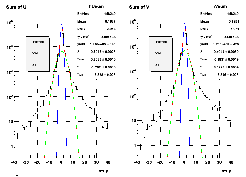
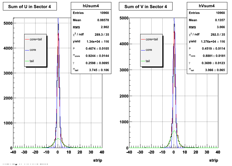
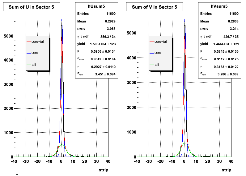
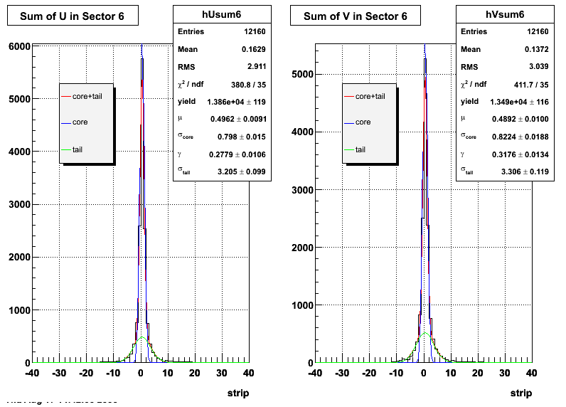
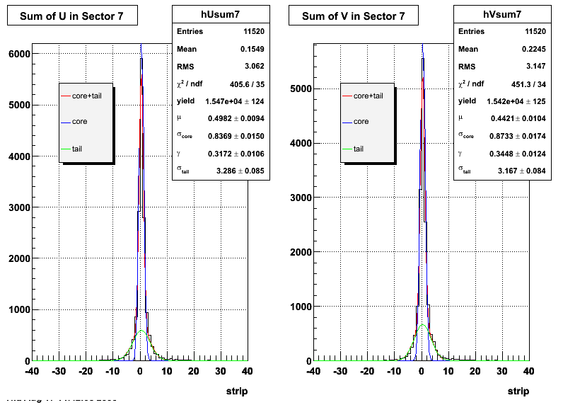
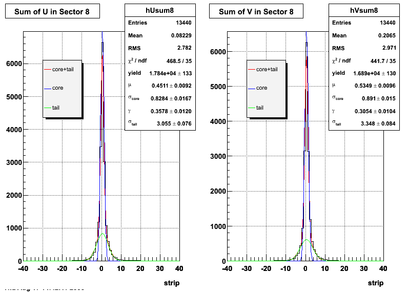
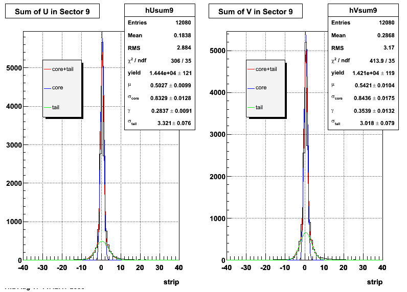
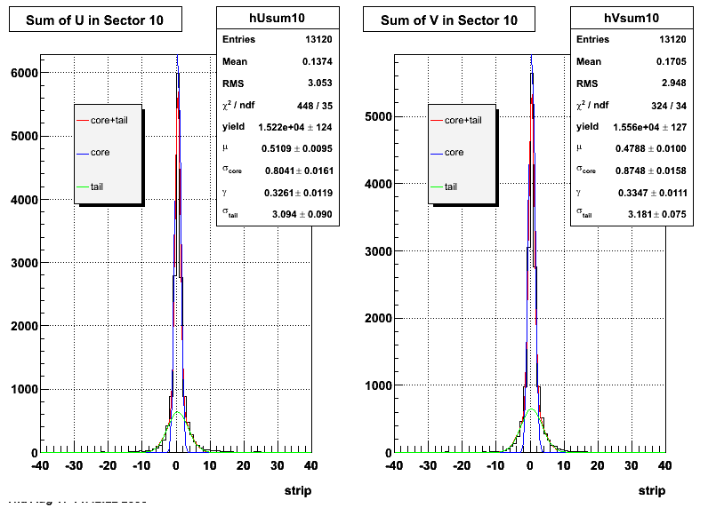
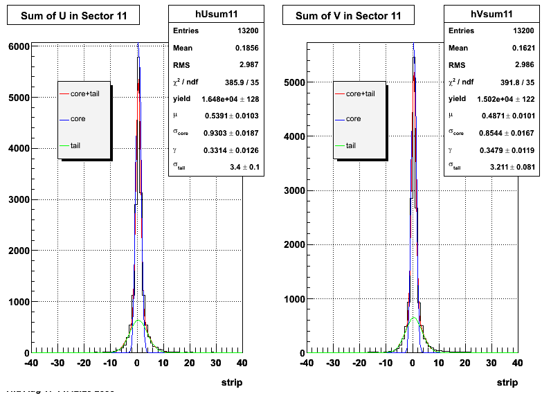
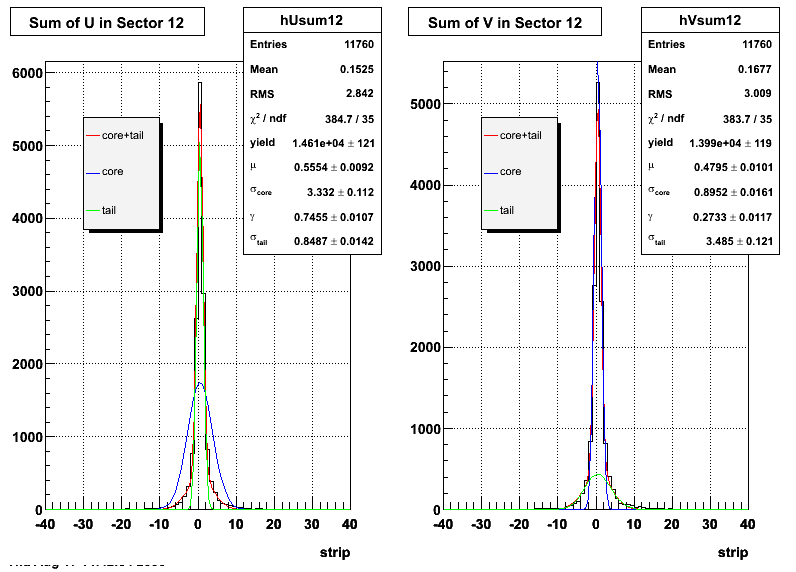
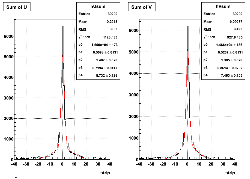
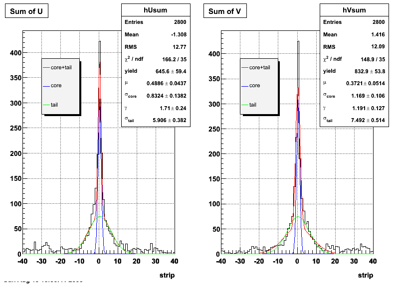
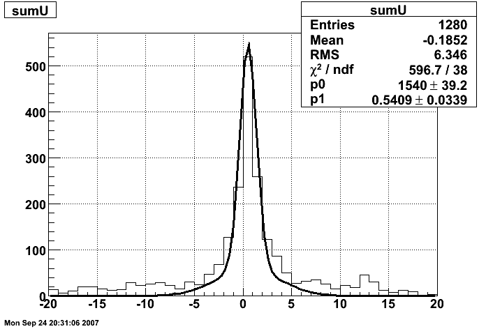
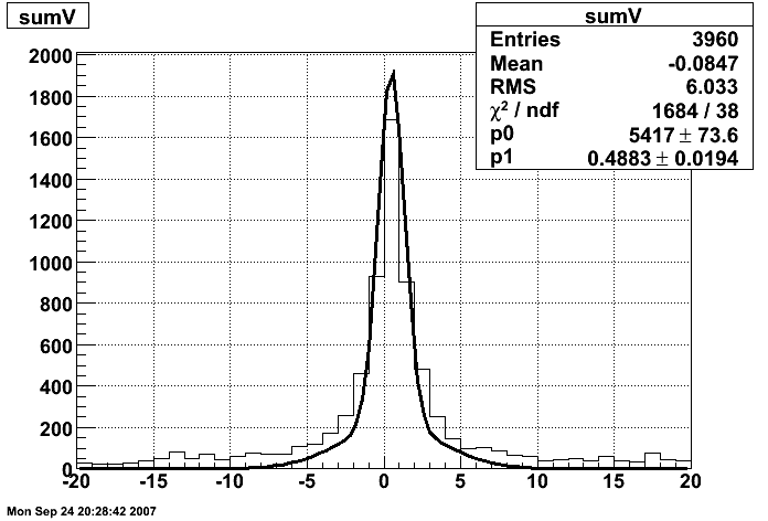
The plots that follow are sums of individual SMD responses in each plane centered around a common mean (here 0), over a +/-40 strips range. The convention for the parameters in the fits below is:

p0=E -- area under the curve which represents energy in MeV
p1=μ -- mean
p2=σ_core -- width of the narrow Gaussian
p3=γ -- relative contribution of the wide Gaussian to the area/height
p4=σ_tail -- width of the wide Gaussian

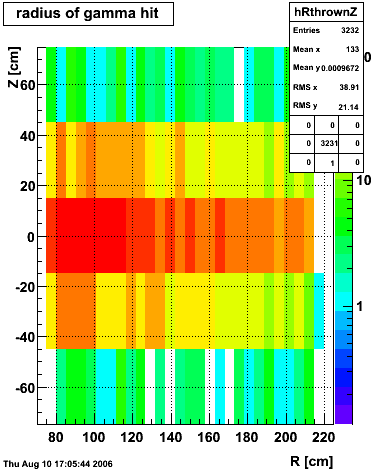
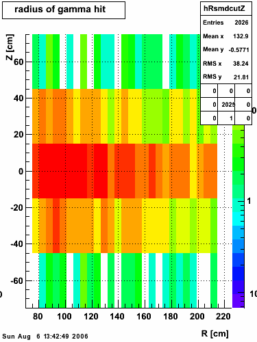
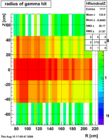
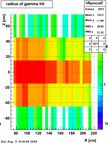
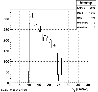
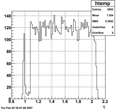
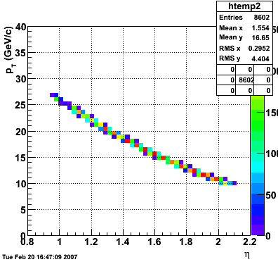
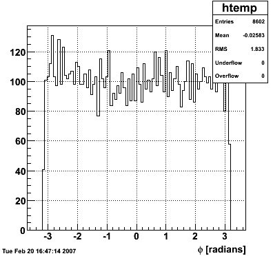
Simulation

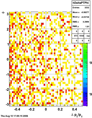
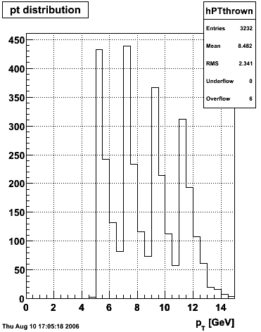
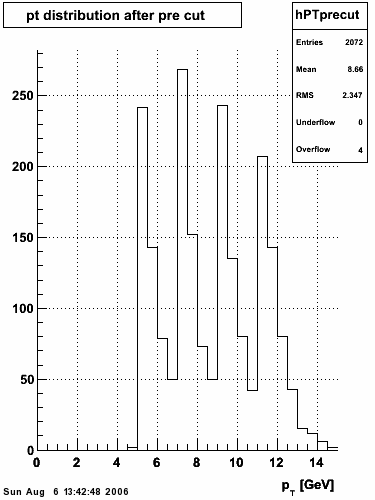
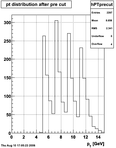
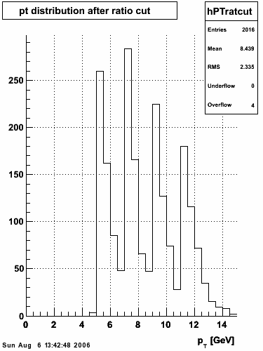
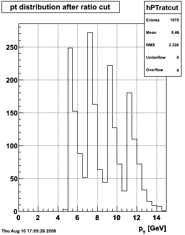
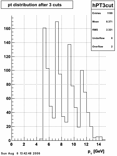
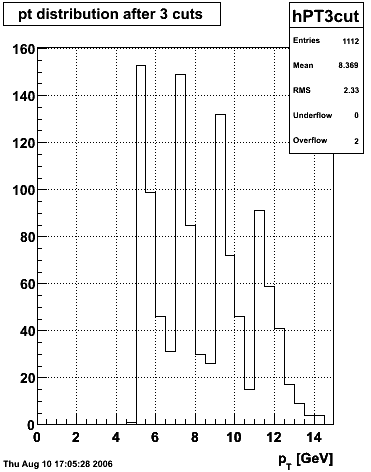
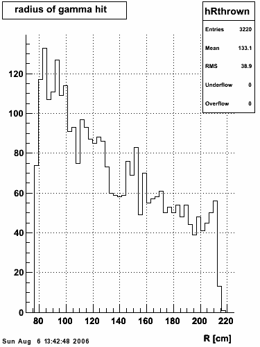
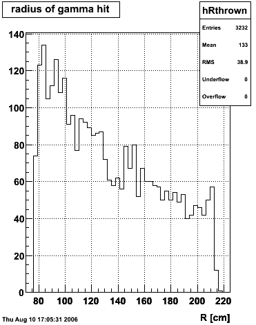
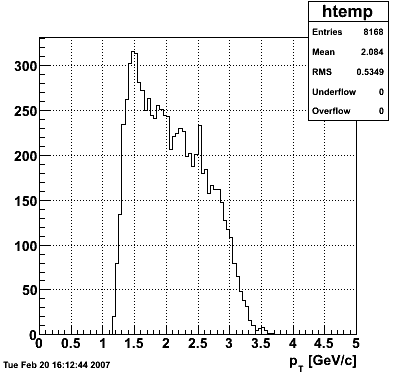
The simulation is from single photons thrown at the EEMC with the following p_T distribution:

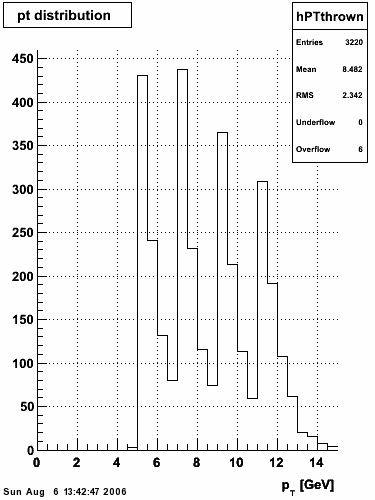
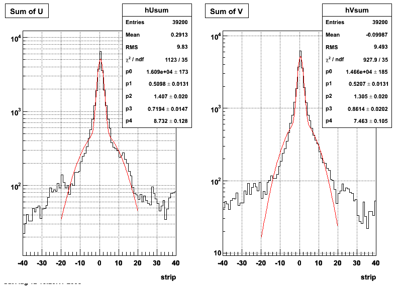
The highest tower above 4 GeV in total energy is selected and the corresponding SMD sector fitted for peaks in both planes, where the area of the peaks in the U plane is constrained to be identical to that of the peak in the V plane. The peak is shifted to be centered at 0 where peaks from other events are then summed. The summed SMD response in each plane is displayed below:

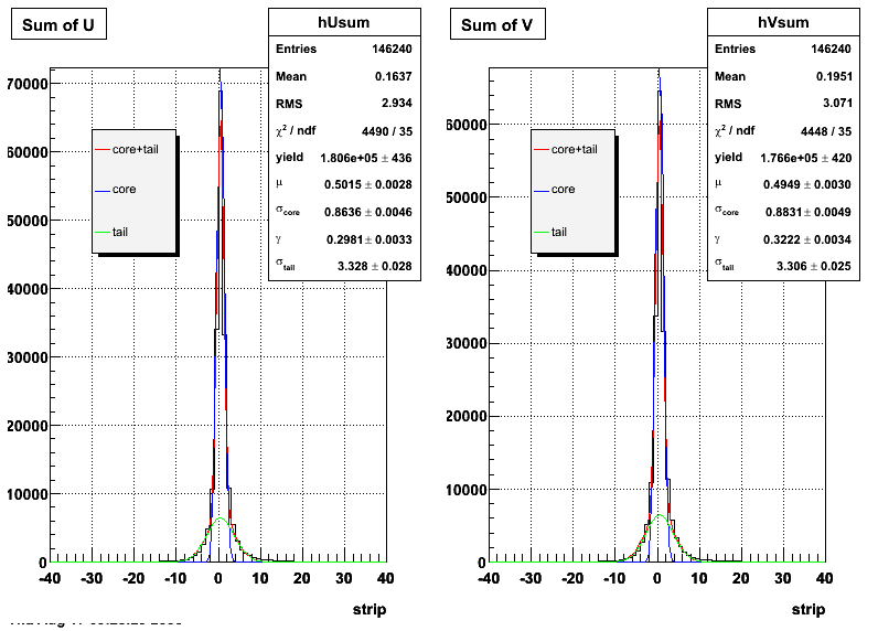
Ditto in log scale.

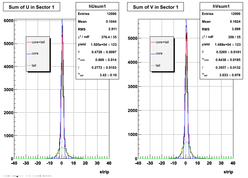
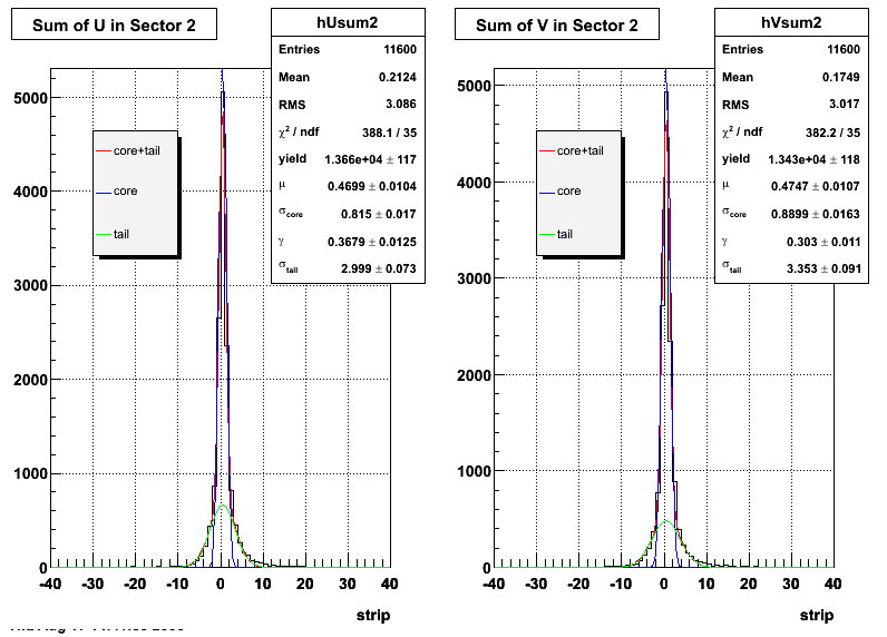
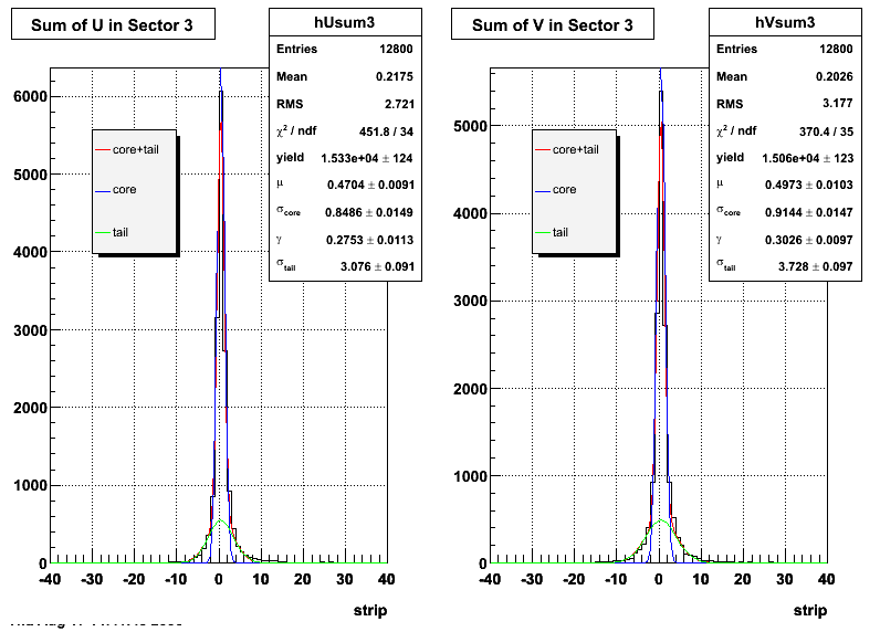
Ditto by sector.

Fit Widths

Sector #	SMD-u σ_core	SMD-u σ_tail	SMD-v σ_core	SMD-v σ_tail
Sector 1	0.869033 ± 0.0142868	3.42031 ± 0.10226	0.84379 ± 0.0185107	3.03287 ± 0.0775009
Sector 2	0.814959 ± 0.0169271	2.99941 ± 0.0730426	0.889892 ± 0.0163065	3.35288 ± 0.0911979
Sector 3	0.84862 ± 0.0148706	3.07648 ± 0.0909689	0.914377 ± 0.014706	3.72821 ± 0.0966915
Sector 4	0.924398 ± 0.0144207	3.74458 ± 0.10611	0.888146 ± 0.0180771	3.06618 ± 0.0647075
Sector 5	0.934218 ± 0.0163887	3.45149 ± 0.0944309	0.911209 ± 0.0175273	3.28633 ± 0.0890581
Sector 6	0.797976 ± 0.0148133	3.20464 ± 0.0986085	0.822437 ± 0.018835	3.30595 ± 0.118813
Sector 7	0.836936 ± 0.0150085	3.28589 ± 0.0853598	0.873338 ± 0.0173883	3.16654 ± 0.0838938
Sector 8	0.828403 ± 0.0167005	3.05517 ± 0.075584	0.891045 ± 0.0152102	3.34806 ± 0.0836394
Sector 9	0.832881 ± 0.0127855	3.3214 ± 0.0762928	0.8436 ± 0.0175466	3.0183 ± 0.079444
Sector 10	0.804059 ± 0.0160906	3.0943 ± 0.0897946	0.874845 ± 0.015788	3.18113 ± 0.0748357
Sector 11	0.930286 ± 0.0187086	3.40024 ± 0.0951671	0.854395 ± 0.0167265	3.21076 ± 0.0812402
Sector 12	3.33227 ± 0.111911	0.848668 ± 0.0142344	0.895174 ± 0.0160939	3.48527 ± 0.12061

Data from 2005 pp200 EEMC HT 1 and 2 triggers

In this sample, high tower triggers, eemc-ht1-mb (96251) and eemc-ht2-mb (96261), from the 2005 p+p at √s=200 GeV ppProduction are selected. The highest tower above 4 GeV is chosen and the corresponding SMD sector is searched for peaks in both planes. Peaks from several events are summed together taking care of shifting them around to have a common mean.

Ditto in log scale.

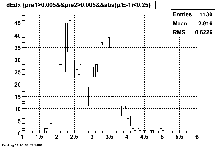
Data from 2005 pp200 electrons

Here, I try to pick a representative sample of electrons from the 2005 pp200 dataset. The cuts used to pick out electrons are:

E_preshower1 > 5 MeV
E_preshower2 > 5 MeV
0.75 < p/E_tower < 1.25
3 < dE/dx < 4 keV/cm

The selection for electrons is illustrated in the dE/dx plot below, where the pions should be on the left and the electrons on the right.

Pibero Djawotho

Last modified Tue Aug 15 10:41:19 EDT 2006

2007.02.05 Reconstructed/Monte Carlo Photon Energy

Reconstructed/Monte Carlo Photon Energy

This study is motivated by Weihong's photon energy loss study where an eta-dependence of reconstructed photon energy to generated photon energy in EEMC simulation was observed.

In this study, the eta-dependence is investigated by running the EEMC slow simulator with the new readjusted weights for the preshower and postshower layers of the EEMC. Details on this are here.

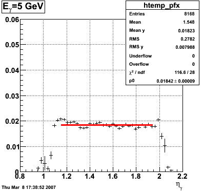
Fit to a constant

Fit to a line

Fit to a quadratic

Comparison between Weihong's and Pibero's results

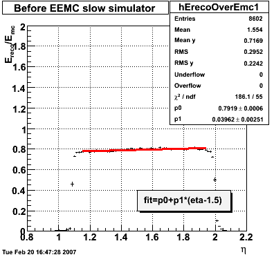
The parameters from the fits are used to plot the fit functions for comparison between Weihong's and Pibero's results.

Constant

Linear

Quadratic

Conclusion

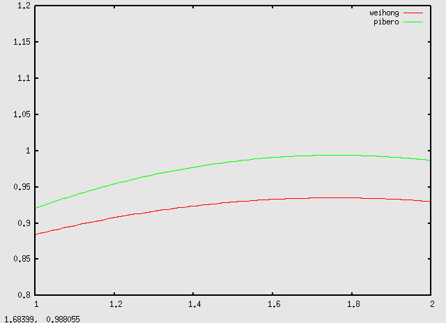
While the adjusted weights for the different EEMC layers contribute to bringing the ratio of reconstructed energy to generated energy closer to unity, they do not remove the eta-dependence.

References

Pibero Djawotho

Last updated Mon Feb 5 10:10:42 EST 2007

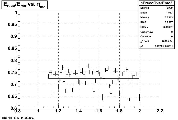
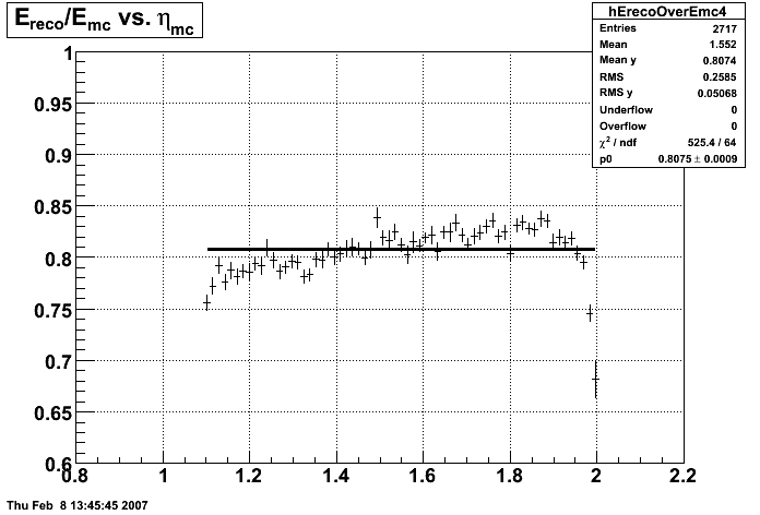
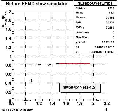
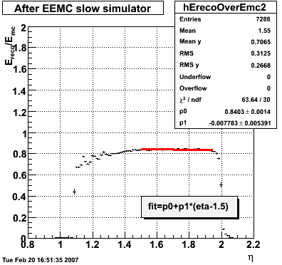
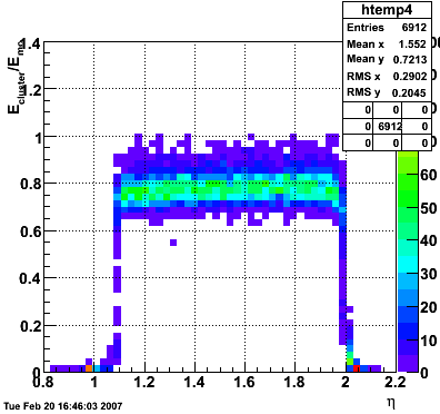
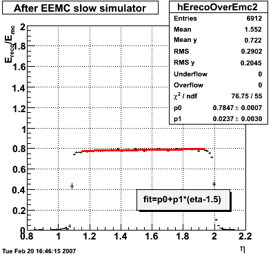
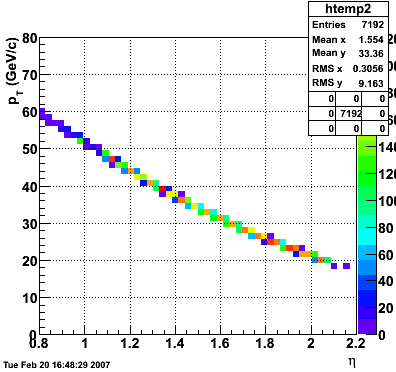
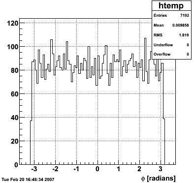
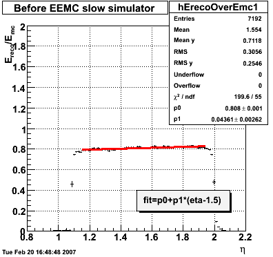
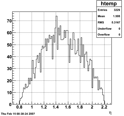
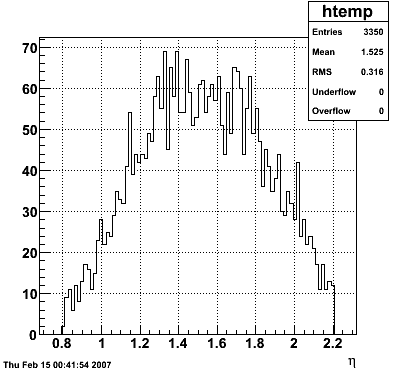
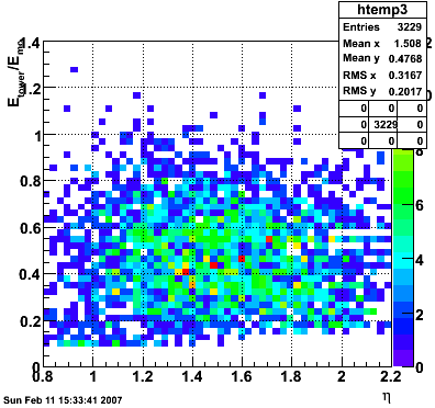
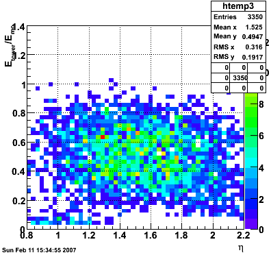
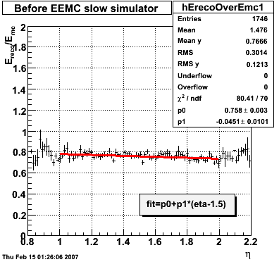
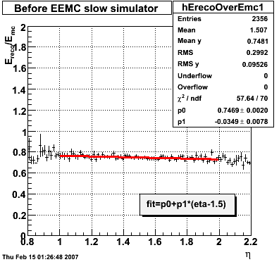
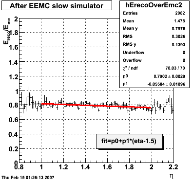
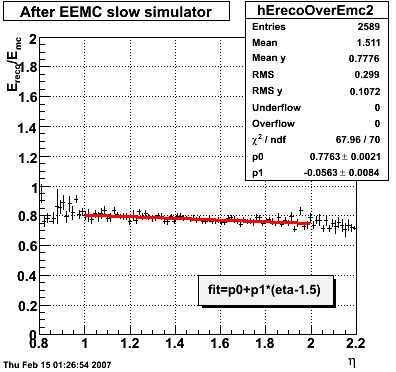
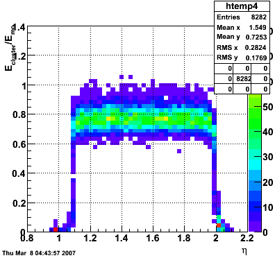
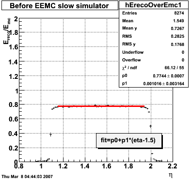
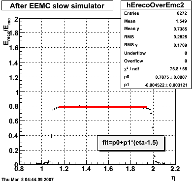
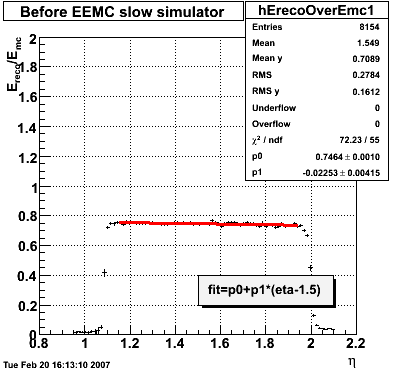
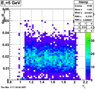
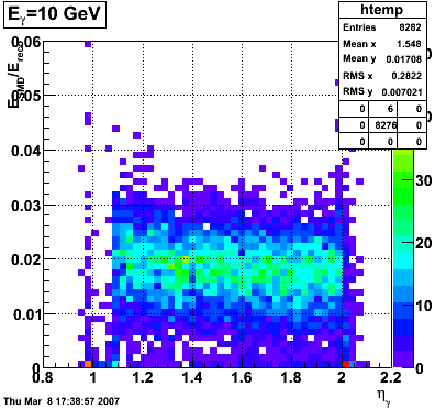
2007.02.08 E_reco / E_mc vs. eta

E_reco / E_mc vs. eta

Legend

black curve: before EEMC slow simulator
red curve: after EEMC slow simulator

Jason's Monte Carlo

4.4k single gamma's
No SVT
Nominal vertex
Flat in pt 4-12 GeV

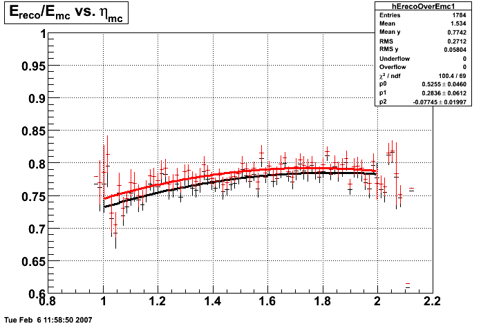
Will's Monte Carlo

10k single gamma's
SVT/SSD out
Vertex at 0
Flat in pt 5-60 GeV

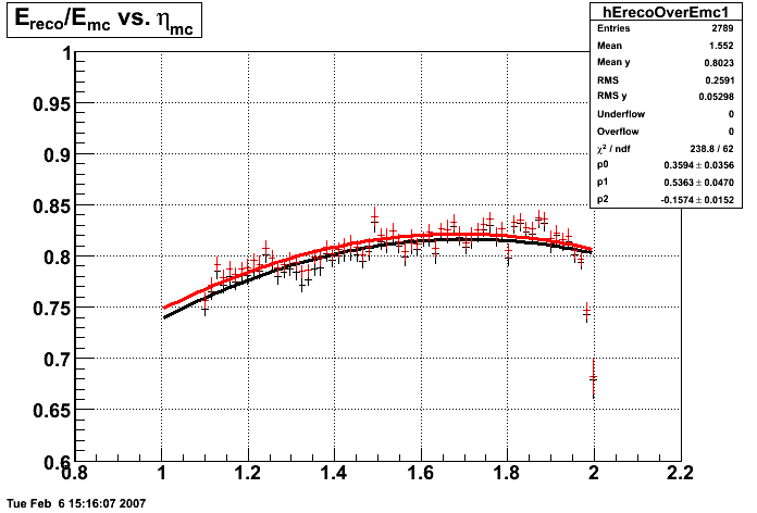
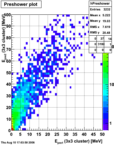
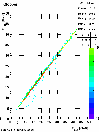
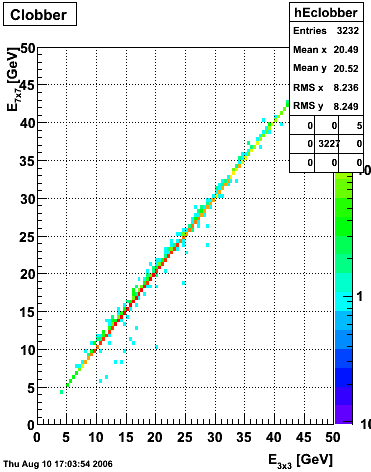
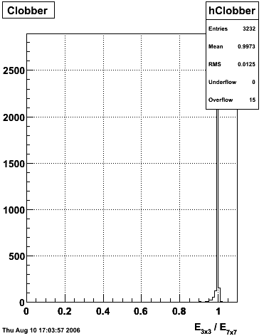
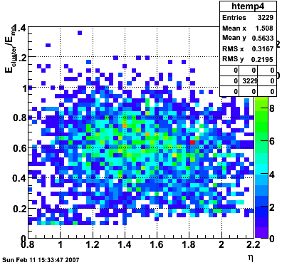
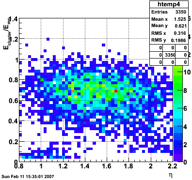
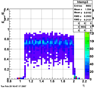
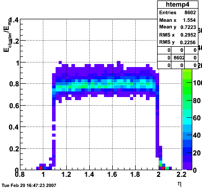
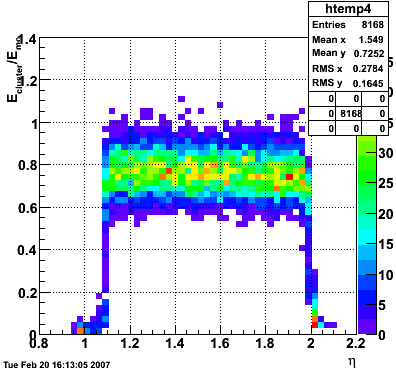
In the plot below, I use the energy of the single tower (tower with max energy) presumably the tower the photon hit. The nonlinearity seems to disappear.

In the plot below, I use the energy of the 3x3 cluster of tower centered around the tower with the max energy. The nonlinearity is restored.

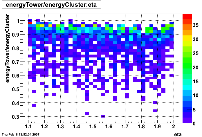
The plot below shows E_tower/E_cluster vs. eta where the cluster consists of 3x3 towers centered around the max energy tower.

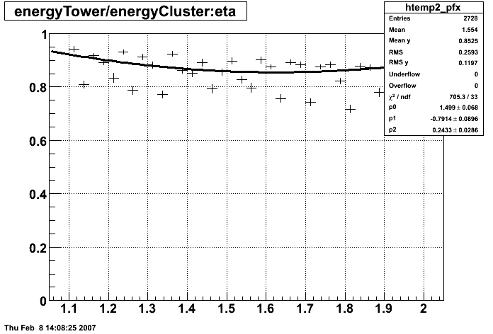
Below is the profile of E_tower/E_cluster vs. eta.

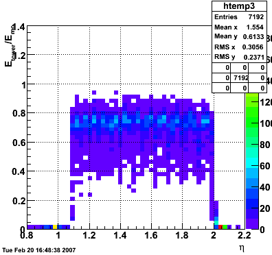
The plot below shows the energy sampled by the entire calorimeter as a function of eta, i.e. sampling fraction as a function of eta.

Sampling fraction integrated over all eta's.

Pibero Djawotho

Last updated Thu Feb 8 13:59:29 EST 2007

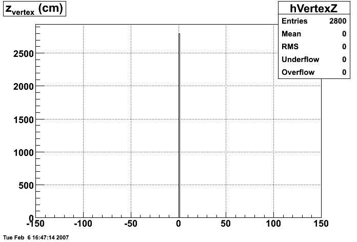
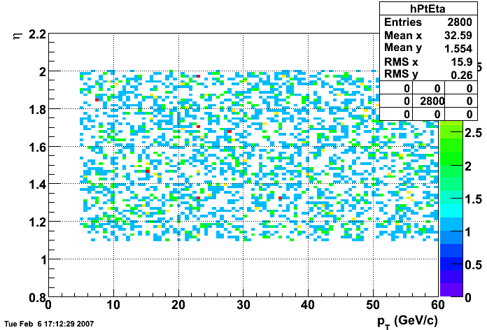
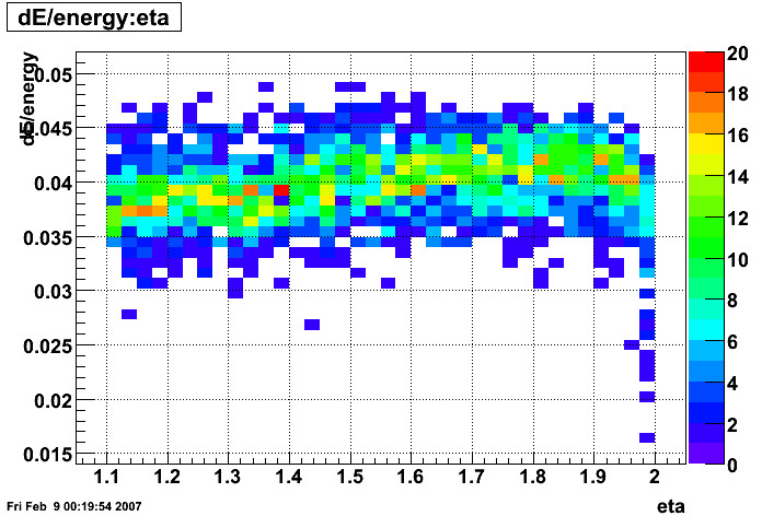
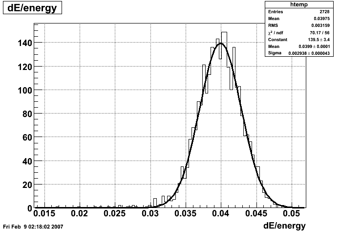
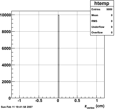
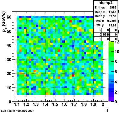
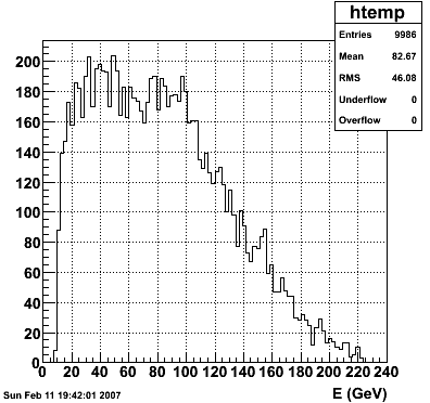
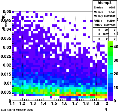
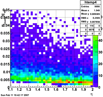
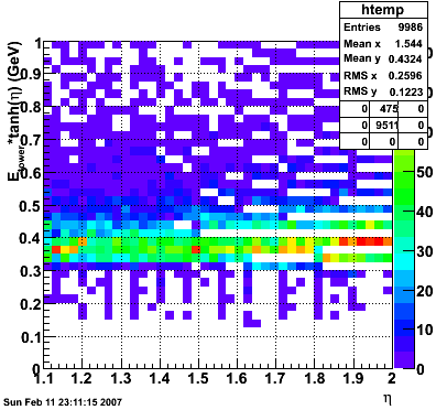
2007.02.11 Reconstructed/Monte Carlo Muon Energy

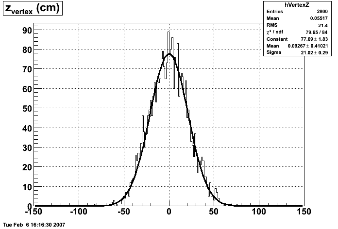
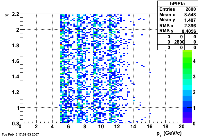
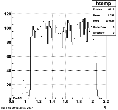
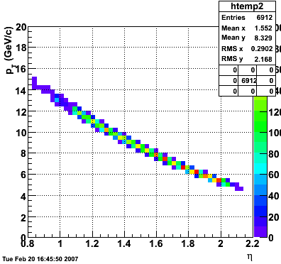
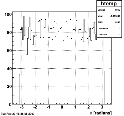
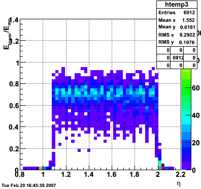
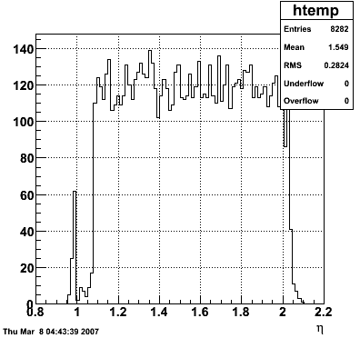
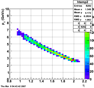
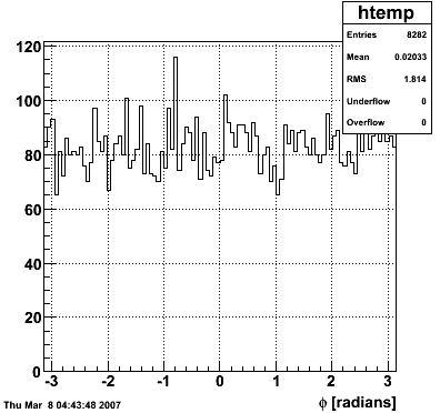
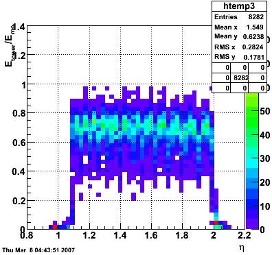
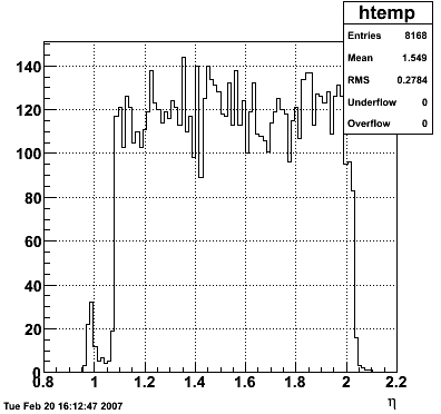
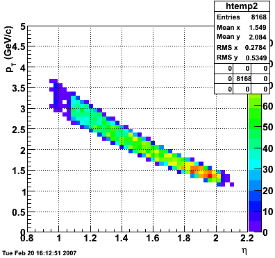
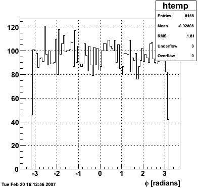
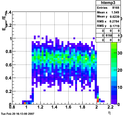
Reconstructed/Monte Carlo Muon Energy

10k muons thrown by Will with:

z_vertex=0
Flat in p_T 5-60 GeV/c
Flat in η 1.1-2

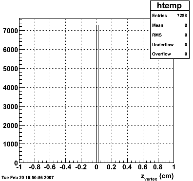
z_vertex

p_T vs. η

E_MC

E_tower/E_MC vs. η

E_cluster/E_MC vs. η

E_towertanh(eta) vs. eta

Pibero Djawotho

Last modified Sun Feb 11 19:51:55 EST 2007

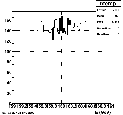
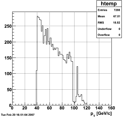
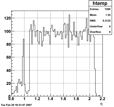
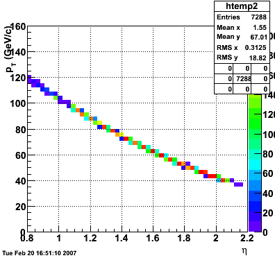
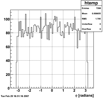
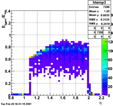
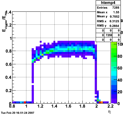
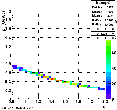
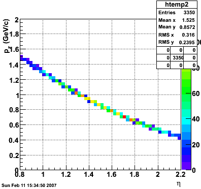
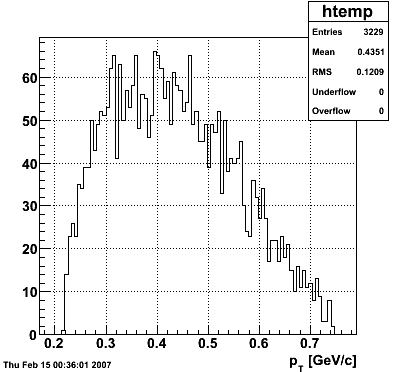
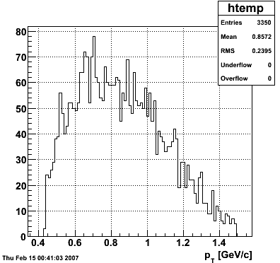
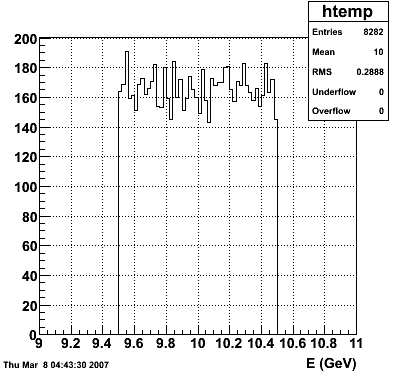
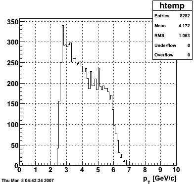
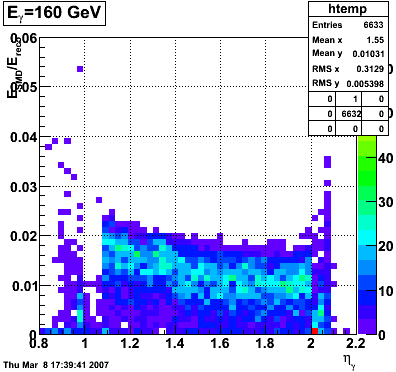
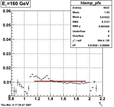
2007.02.15 160 GeV photons

160 GeV photons

10k 160 GeV photons
z_vertex=0
η range 0.8-2.2
SVT/SSD out

Pibero Djawotho

Last updated Thu Feb 15 04:33:09 EST 2007

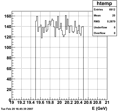
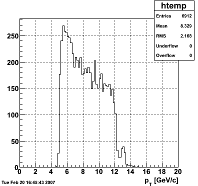
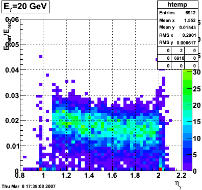
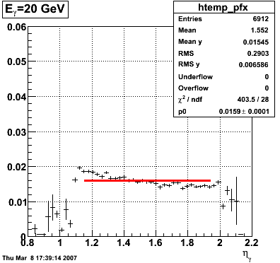
2007.02.15 20 GeV photons

20 GeV photons

10k 20 GeV photons
z_vertex=0
η range 0.8-2.2
SVT/SSD out

Pibero Djawotho

Last updated Thu Feb 15 04:32:25 EST 2007

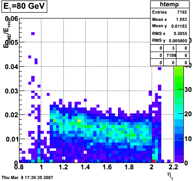
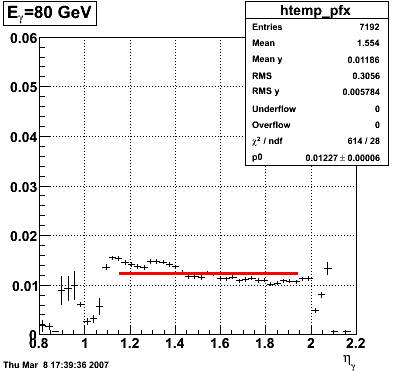
2007.02.15 80 GeV photons

80 GeV photons

10k 80 GeV photons
z_vertex=0
η range 0.8-2.2
SVT/SSD out

Pibero Djawotho

Last updated Thu Feb 15 03:16:54 EST 2007

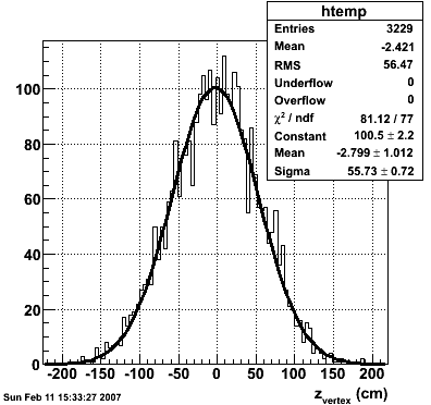
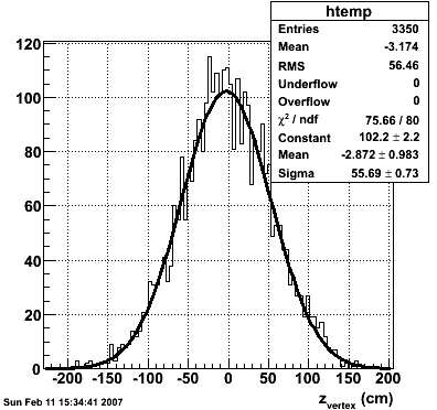
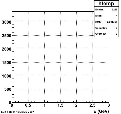
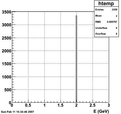
2007.02.15 Reconstructed/Monte Carlo Electron Energy

Reconstructed/Monte Carlo Electron Energy

E=1 GeV	E=2 GeV

Pibero Djawotho

Last modified Thu Feb 15 00:42:30 EST 2007

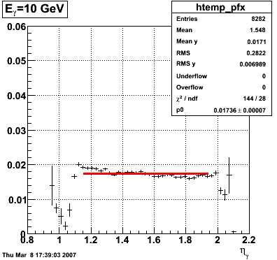
2007.02.19 10 GeV photons

10 GeV photons

10k 10 GeV photons
z_vertex=0
η range 0.8-2.2
SVT/SSD out

Pibero Djawotho

Last updated Mon Feb 19 20:35:13 EST 2007

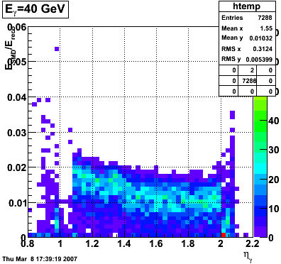
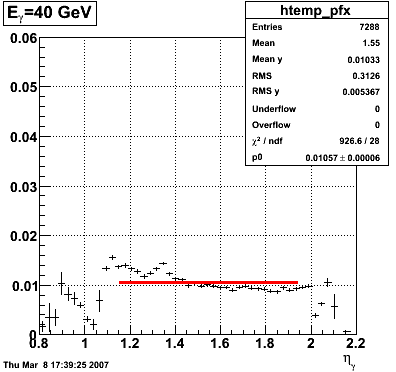
2007.02.19 40 GeV photons

40 GeV photons

10k 40 GeV photons
z_vertex=0
η range 0.8-2.2
SVT/SSD out

Pibero Djawotho

Last updated Mon Feb 19 20:37:37 EST 2007

2007.02.19 5 GeV photons

5 GeV photons

10k 5 GeV photons
z_vertex=0
η range 0.8-2.2
SVT/SSD out

Pibero Djawotho

Last updated Mon Feb 19 20:13:39 EST 2007

2007.02.19 Summary of Reconstructed/Monte Carlo Photon Energy

Summary of Reconstructed/Monte Carlo Photon Energy

Description

The study presented here uses Monte Carlo data sets generated by Will Jacobs at different photon energies (5, 10, 20, 40, 80, 160 GeV):

10k photons
vertex at 0
eta 0.8-2.2
SVT/SSD out

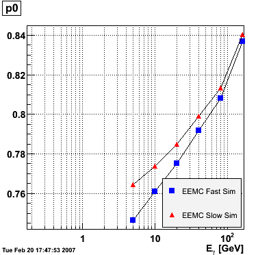
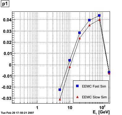
For each photon energy, the ratio E_reco/E_MC vs. eta was plotted and fitted to the function p0+p1*(1-eta), where E_reco is the reconstructed photon energy integrated over the

entire

EEMC. The range of the fit was fixed from 1.15 to 1.95 to avoid EEMC edge effects. The advantage of parametrizing the eta-dependence of the ratio in this way is that p0 is immediately interpretable as the ratio in the middle of the EEMC. The parameters p0 and p1 vs. photon energy were subsequently plotted for the EEMC fast and slow simulator.

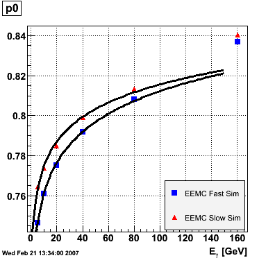
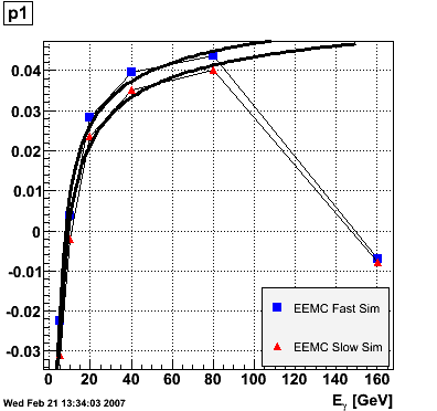
EEMC Fast/Slow Simulator Results

Conclusions

The parameter p0, i.e. the ratio E_reco/E_MC in the mid-region of the EEMC, increases monotonically from 0.74 at 5 GeV to 0.82 at 160 GeV, and the parameter p1, i.e. the slope of the eta-dependence, also increases monotonically from -0.035 at 5 GeV to 0.038 at 160 GeV. There appears to be a magic energy around 10 GeV where the response of the EEMC is nearly flat across its entire pseudorapidity range. The anomalous slope p1 at 160 GeV for the EEMC slow simulator is an EEMC hardware saturation effect. The EEMC uses 12-bit ADC's for reading out tower transverse energies and is set for a 60 GeV range. Any particle which deposits more than 60 GeV in E_T will be registered as depositing only 60 GeV as the ADC will return the maximum value of 4095. This translates into a limit on the eta range of the EEMC for a particular energy. Let's say that energy is 160 GeV and the EEMC tops at 60 GeV in E_T, then the minimum eta is acosh(160/60)=1.6. This limitation is noticeable in a plot of E_reco/E_MC vs. eta. This anomaly is not observed in the result of the EEMC fast simulator because the saturation behavior was not implemented at the time of the simulation (it has since been corrected). The energy-dependence of the parameter p0 is fitted to p0(E)=a+b*log(E) and the parameter p1 to p1(E)=a+b/log(E). The results are summarized below:

EEMC fast simulator fit p0(E)=a+b*log(E)
a = 0.709946 +/- 0.00157992
b = 0.022222 +/- 0.000501239

EEMC slow simulator fit p0(E)=a+b*log(E)
a = 0.733895 +/- 0.00359237
b = 0.0177537 +/- 0.0011397

EEMC fast simulator fit p1(E)=a+b/log(E)
a = 0.0849103 +/- 0.00556979
b = -0.175776 +/- 0.0138241

EEMC slow simulator fit p1(E)=a+b/log(E)
a = 0.0841488 +/- 0.0052557
b = -0.187769 +/- 0.0130445

Pibero Djawotho

Last updated Mon Feb 19 23:18:44 EST 2007

2007.05.24 gamma/pi0 separation in EEMC using linear cut

gamma/pi0 separation in EEMC using linear cut

Pibero Djawotho

Last updated Thu May 24 04:41:13 EDT 2007

2007.05.24 gamma/pi0 separation in EEMC using quadratic cut

gamma/pi0 separation in EEMC using quadratic cut

Pibero Djawotho

Last updated Thu May 24 04:41:13 EDT 2007

2007.05.24 gamma/pi0 separation in EEMC using quadratic cut

gamma/pi0 separation in EEMC using quadratic cut

Pibero Djawotho

Last updated Thu May 24 04:41:13 EDT 2007

2007.05.30 Efficiency of reconstructing photons in EEMC

Efficiency of reconstructing photons in EEMC

Monte Carlo sample

10k photons
STAR y2006 geometry
z-vertex=0
Flat in pt 10-30 GeV
Flat in eta 1.0-2.1

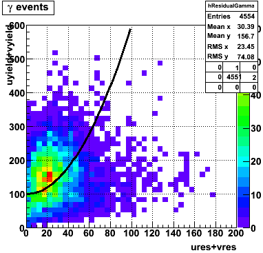
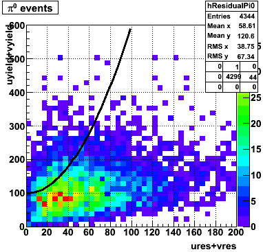
SMD gamma/pi0 discrimination algorithm

The following

slide

from the IUCF STAR Web site gives a brief overview of the SMD gamma/pi0 discrimination algorithm using the method of maximal sided fit residual (data - fit). This technique comes to STAR EEMC from the Tevatron via Les Bland via Jason Webb. The specific fit function used in this analysis is:

f(x)=[0]*(0.69*exp(-0.5*((x-[1])/0.87)**2)/(sqrt(2*pi)*0.87)+0.31*exp(-0.5*((x-[1])/3.3)**2)/(sqrt(2*pi)*3.3))

x is the strip id in the SMD-u or SMD-v plane. The widths of the narrow and wide Gaussians are determined from empirical fits of shower shape response in the EEMC from simulation.

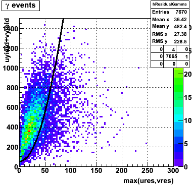
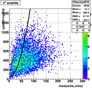
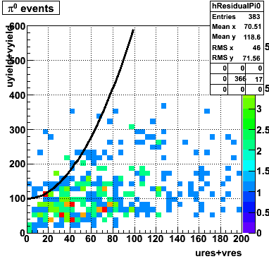
Optimizing cuts for gamma/pi0 separation

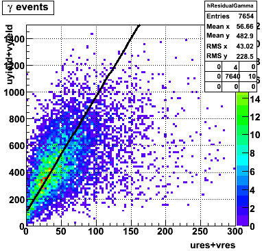
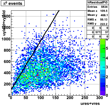
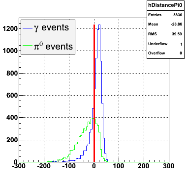
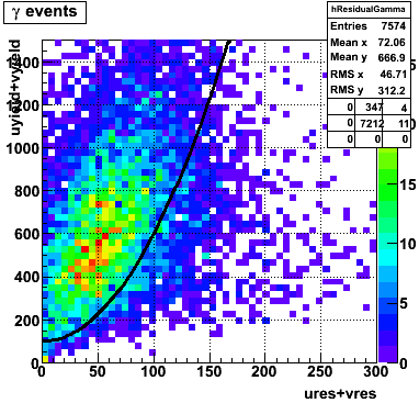
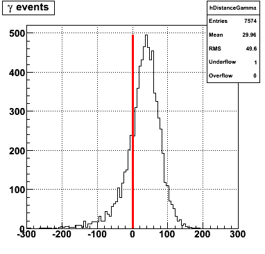
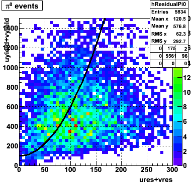
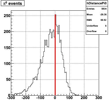
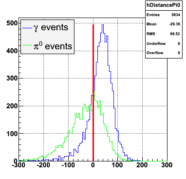
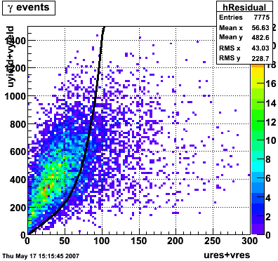
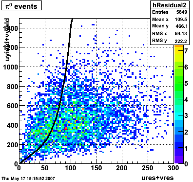
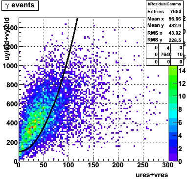
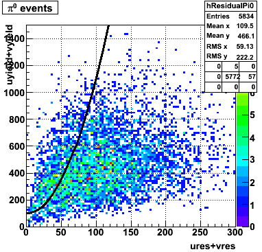
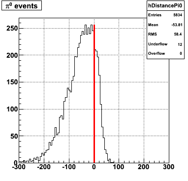
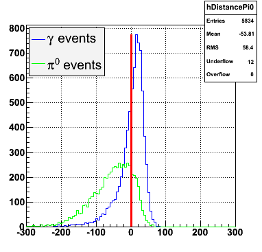
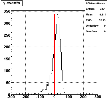
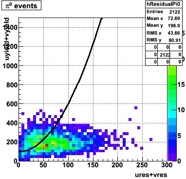
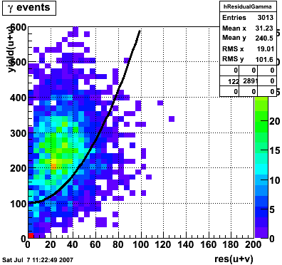
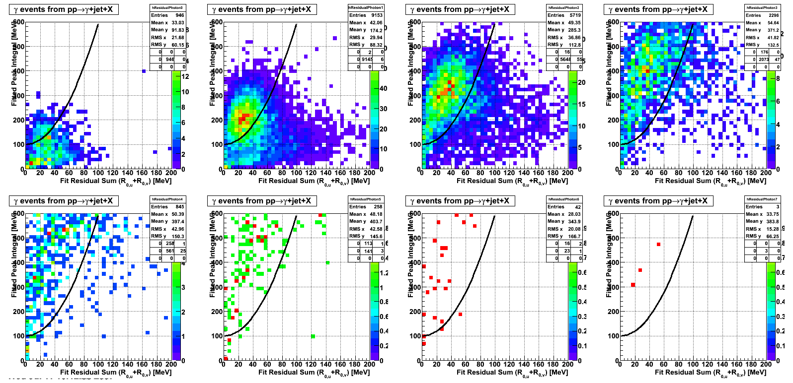
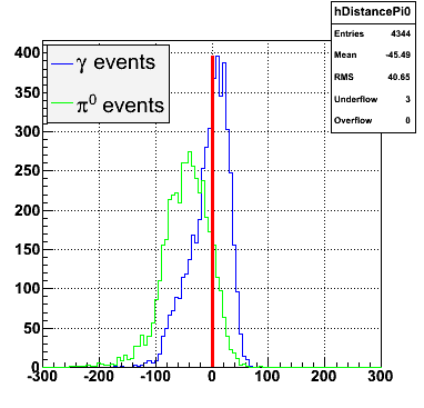
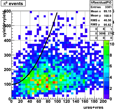
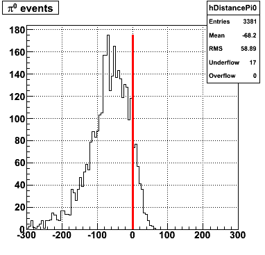
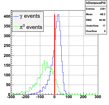
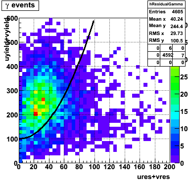
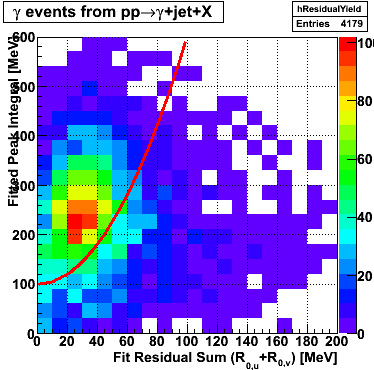
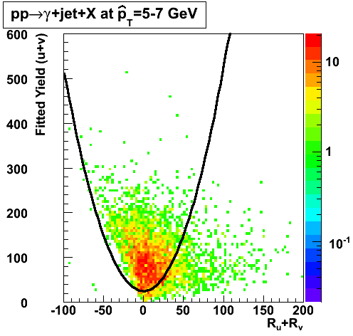
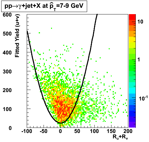
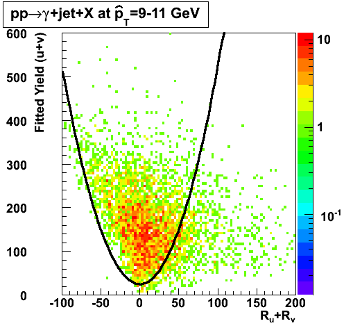
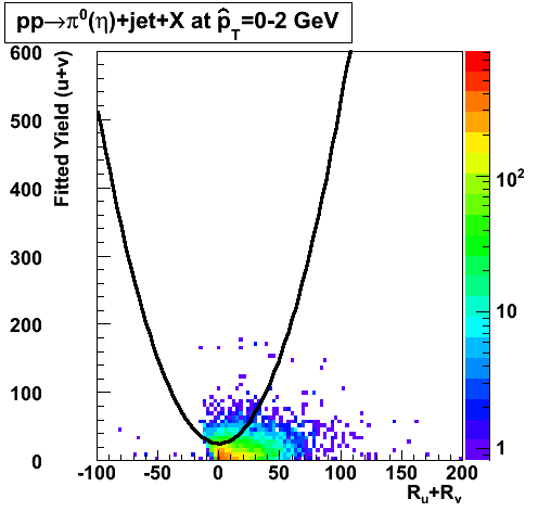
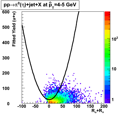
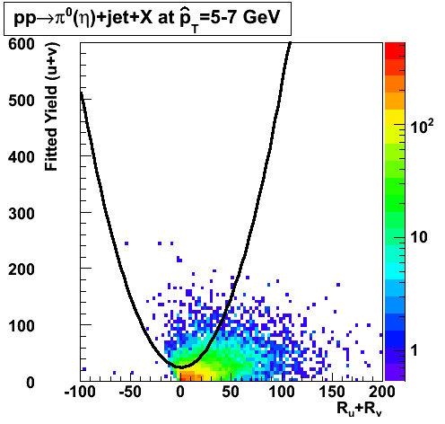
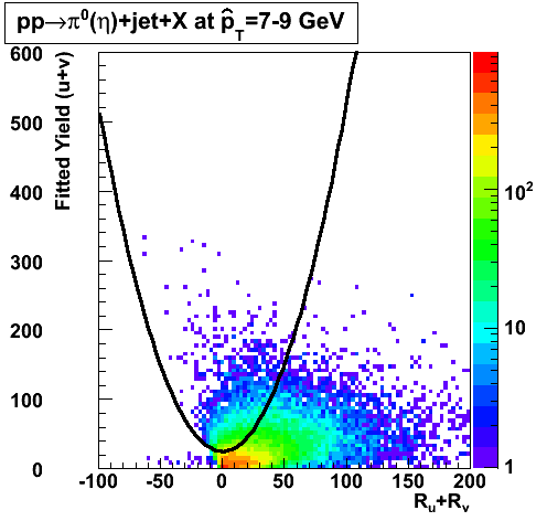
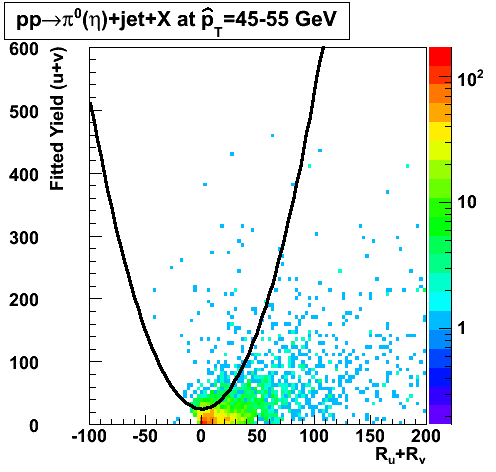
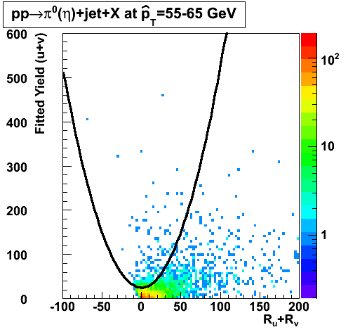
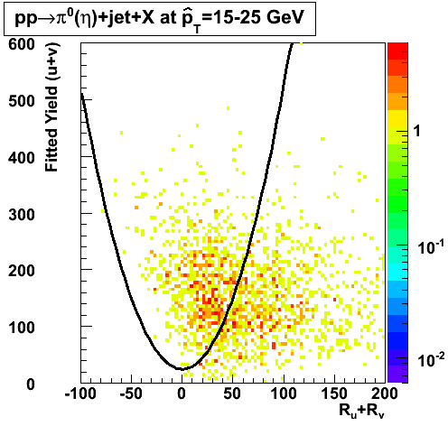
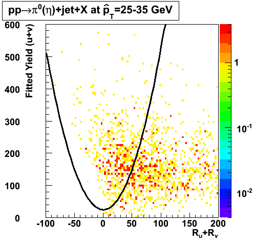
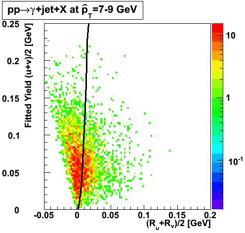
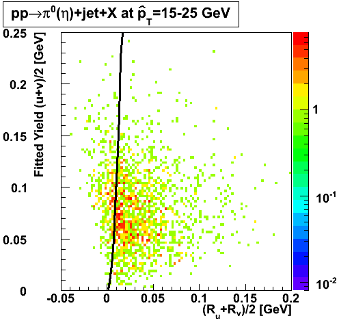
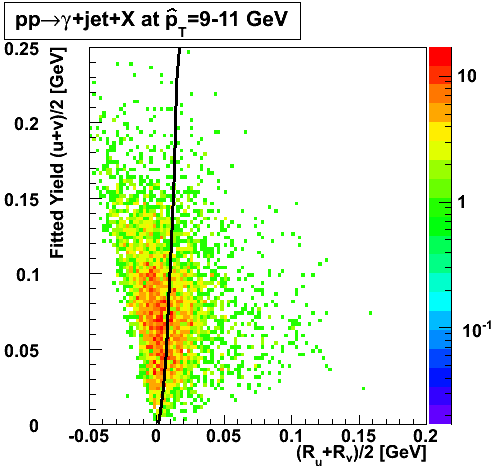
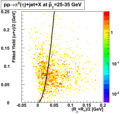
In the rest of this analysis, only those photons which have reconstructed pt > 5 GeV are kept. There is no requirement that the photon doesn't convert. The dividing curve between photons and pions is:

f(x)=4*x+1e-7*x**5

The y-axis is integrated yield over the SMD-u and SMD-v plane, and the x-axis is the sum of the maximal sided residual of the SMD-u and SMD-v plane.

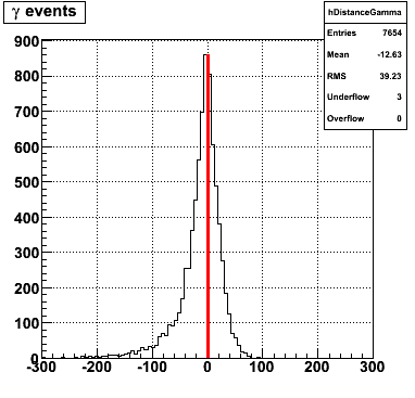
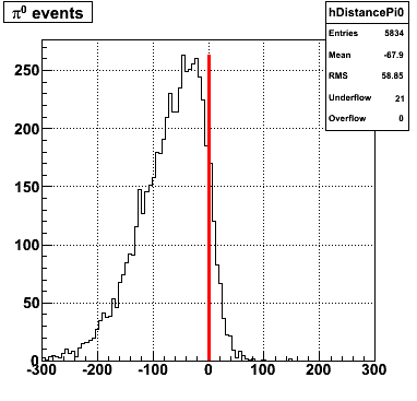
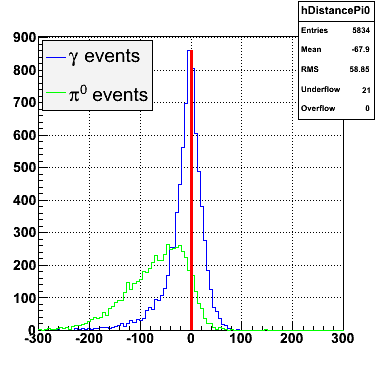
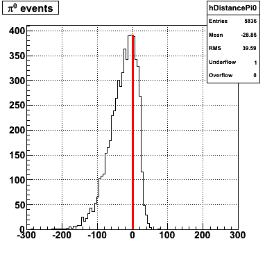
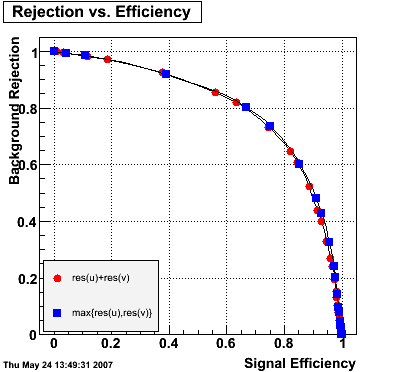
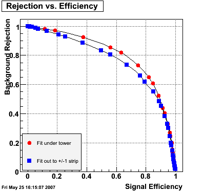
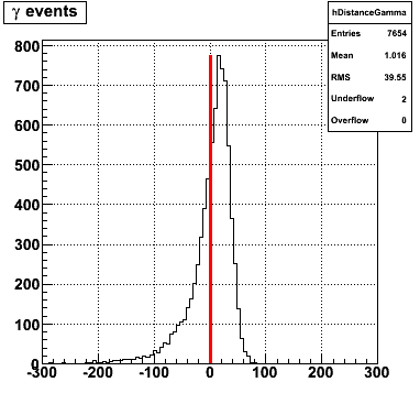
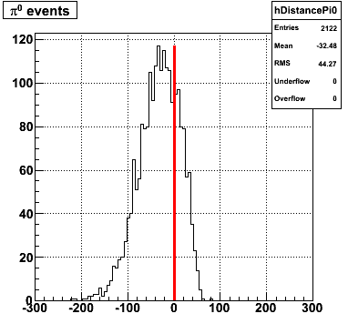
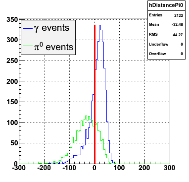
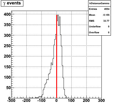
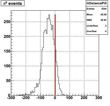
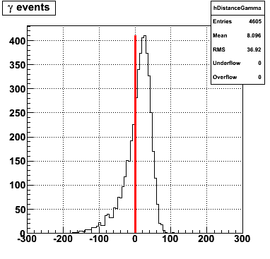
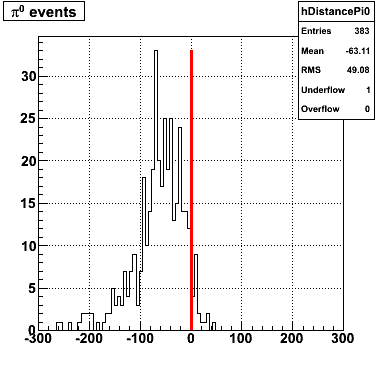
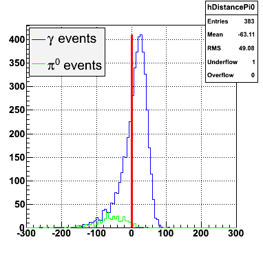
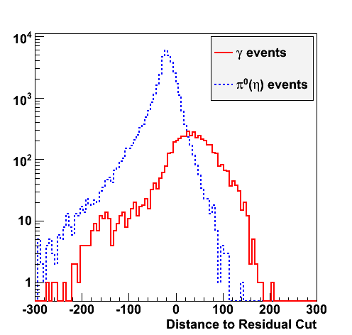
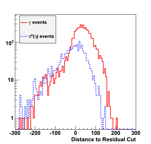
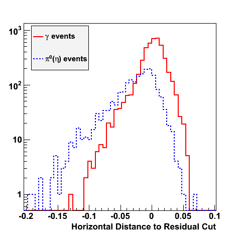
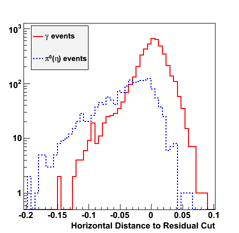
Following exchanges with Scott Wissink, the idea is to move from a quintic to a quadratic to reduce the number of parameters. In addition, the perpendicular distance between the curve and a point in the plane is used to estimate the likelihood of a particle being a photon or pion. Distances above the curve are positive and those below are negative. The more positive the distance, the more likely the particle is a photon. The more negative the distance, the more likely the particle is a pion.

Hi Pibero,

With your new "linear plus quintic" curve (!) ... how did you choose the
coefficients for each term?  Or even the form of the curve?  I'm not
being picky, but how to optimize such curves will be an important issue
as we (hopefully soon) move on to quantitative comparisons of efficiency
vs purity.

As a teaser, please see attached - small loss of efficiency, larger gain
in purity.

Scott

Hi Pibero,

I just worked out the distance of closest approach to a curve of the form

    y(x) = a + bx^2

and it involves solving a cubic equation - so maybe not so trivial after
all.  But if you want to pursue this (not sure it is your highest
priority right now!), the cubic could be solved numerically and "alpha"
could be easily calculated.

More fun and games.

Scott

Hi Pibero,

I played around with the equations a bit more, and I worked out an
analytic solution.  But a numerical solution may still be better, since
it allows more flexibility in the algebraic form of the 'boundary' line
between photons and pions.

Here's the basic idea:  suppose the curved line that cuts between
photons and pions can be expressed as y = f(x).  If we are now given a
point (x0,y0) in the plane, our goal is to find the shortest distance to
this line.  We can call this distance d (I think on your blackboard we
called it alpha).

To find the shortest distance, we need a straight line that passes
through (x0,y0) and is also perpendicular to the curve f(x).  Let's
define the point where this straight line intersects the curve as
(x1,y1).  This means (comparing slopes)

    (y1 - y0) / (x1 - x0) = -1 / f'(x1)

where f'(x1) is the derivative of f(x) evaluated at the point (x1,y1). 
Rearranging this, and using y1 = f(x1), yields the general result

    f(x1) f'(x1)  -  y0 f'(x1)  +   x1  -   x0  =  0

So, given f(x) and the point (x0,y0), the above is an equation in only
x1.  Solve for x1, use y1 = f(x1), and then the distance d of interest
is given by

    d = sqrt[ (x1 - x0)^2 + (y1 - y0)^2 ]

Example:  suppose we got a reasonable separation of photons and pions
using a curve of the form

    y = f(x) = a + bx^2

Using this in the above general equation yields the cubic equation

    (2b^2) x1^3  +  (2ab + 1 - 2by0) x1  -  x0  =  0

Dividing through by 2b^2, we have an equation of the form

    x^3 + px + q = 0

This can actually be solved analytically - but as I mentioned, a
numerical approach gives us more flexibility to try other forms for the
curve, so this may be the way to go.  I think (haven't proved
rigorously) that for positive values of the constants a, b, x0, and y0,
the cubic will yield three real solutions for x1, but only one will have
x1 > 0, which is the solution of interest.

Anyway, it has been an interesting intellectual exercise!

Scott

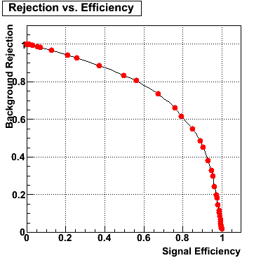
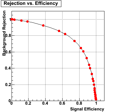
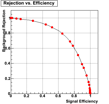
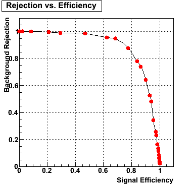
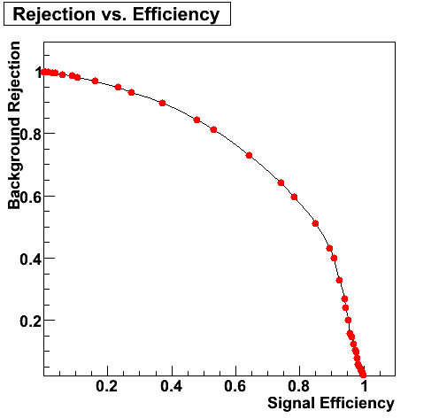
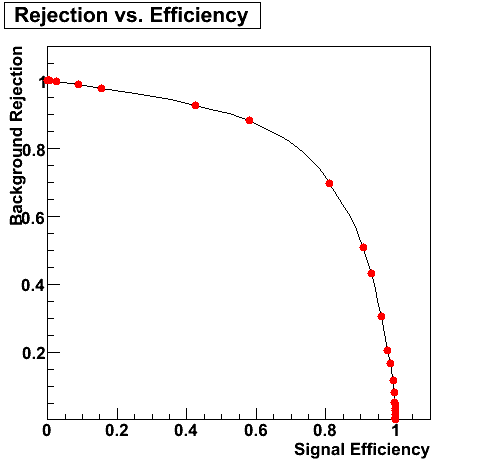
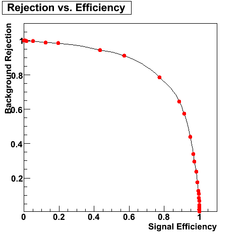
I made use of the ROOT function TMath::RootsCubic to solve the cubic equation numerically for computing distances of each point to the curve. With the new quadratic curve f(x)=100+0.1*x^2 the efficiency is 63% and the rejection is 82%.

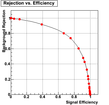
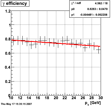
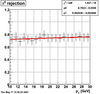
Efficiency and Rejection

The plot on the left below shows the efficiency of identifying photons over the pt range of 10-30 GeV and the one on the right shows the rejection rate of single neutral pions. Both average about 75% over the pt range of interest.

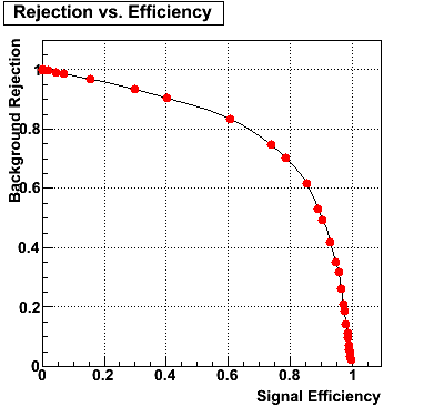
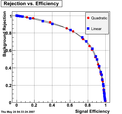
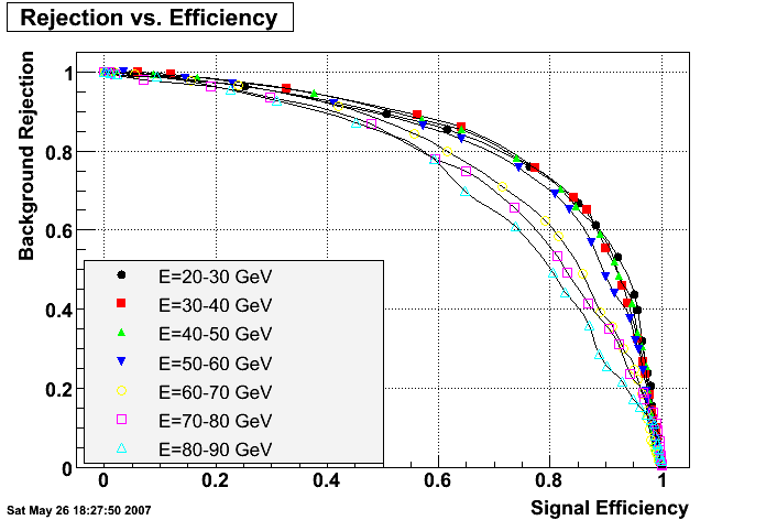
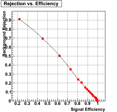
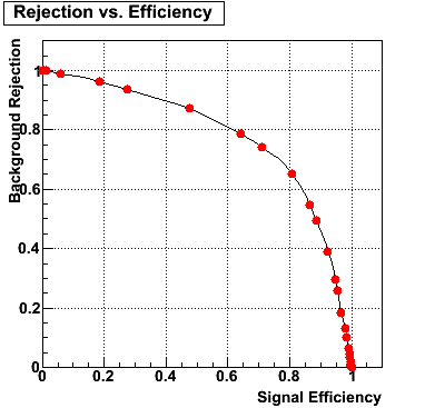
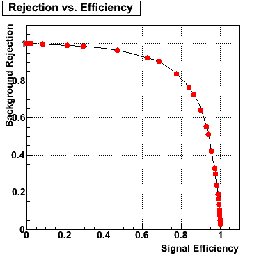
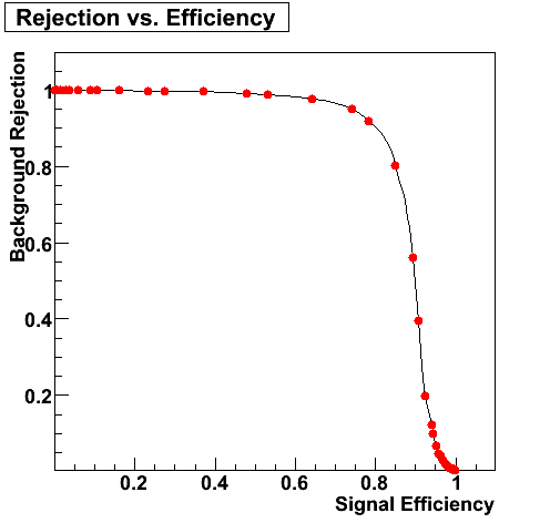
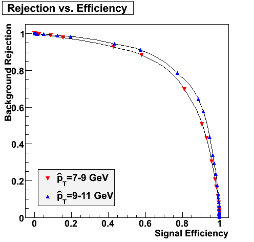
Rejection vs. efficiency at different energies

The plot below shows background rejection vs. signal efficiency for different energy ranges of the thrown gamma/pi0.

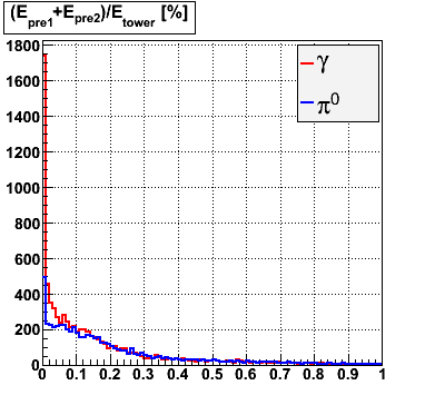
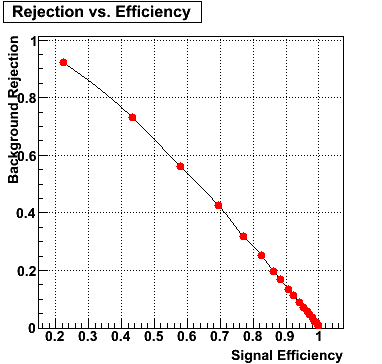
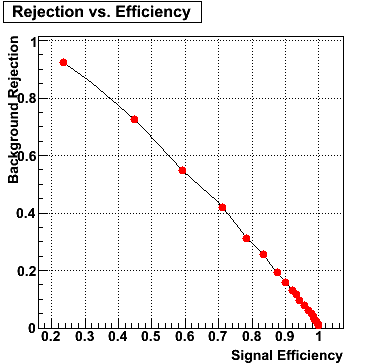
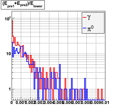
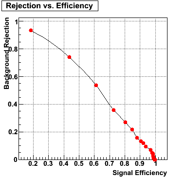
Rejection vs. efficiency with preshower cut

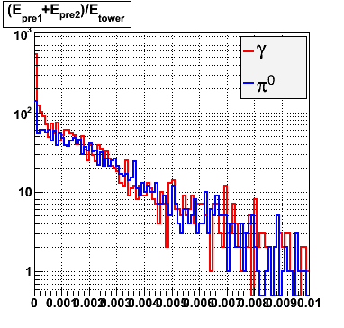
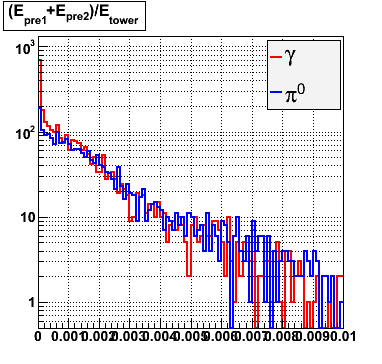
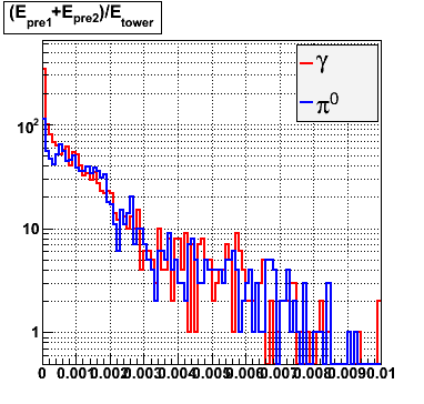
Below on the left is a plot of the ratio of the sum of preshower 1 and 2 to tower energy for both photons (red) and pions (blue). On the right is the rejection of pions vs. efficiency of photons as I cut on the ratio of preshower to tower. It is clear from these plots that the preshower layer is not a good gamma/pi0 discriminator, although can be used to add marginal improvement to the separation preovided by the shower max.

ALL ENERGIES

E=20-40 GeV

E=40-60 GeV

E=60-80 GeV

E=80-90 GeV

Pibero Djawotho

Last updated Wed May 30 00:32:16 EDT 2007

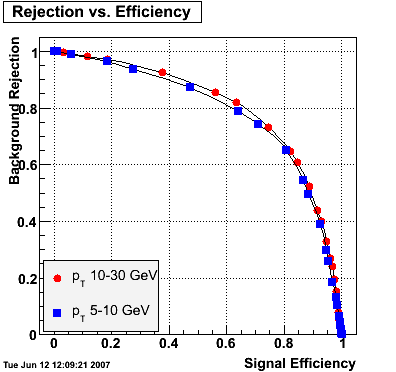
2007.06.12 gamma/pi0 separation in EEMC at pT 5-10 GeV

gamma/pi0 separation in EEMC at pT 5-10 GeV

Pibero Djawotho

Last updated Tue Jun 12 11:59:42 EDT 2007

2007.06.28 Photons in Pythia

Pythia Simulations

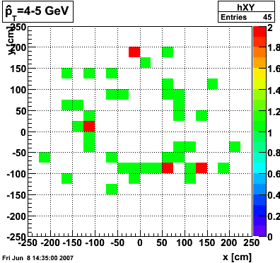
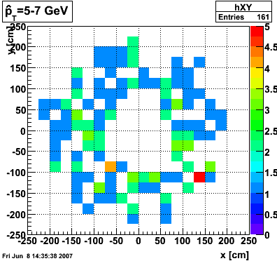
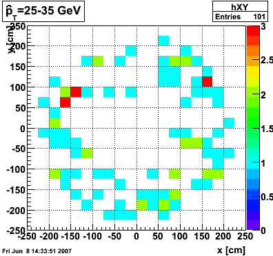
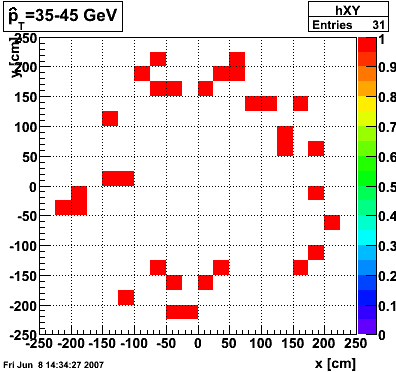
All partonic pT

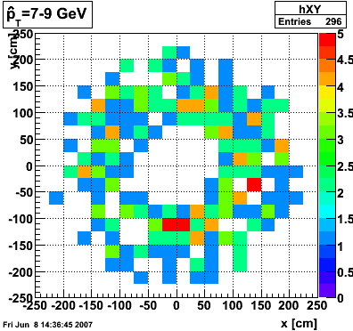
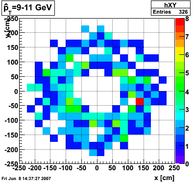
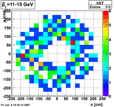
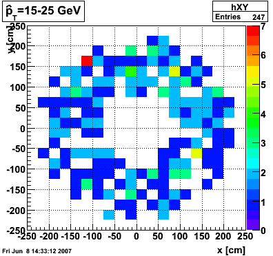
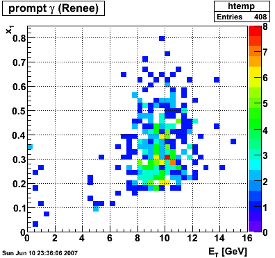
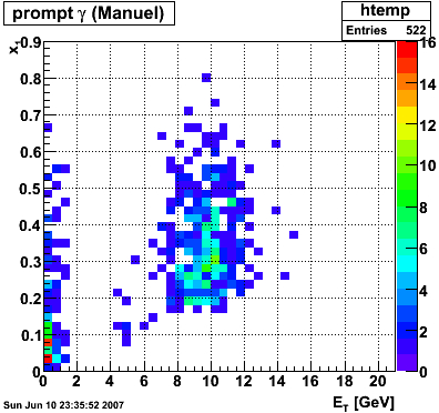
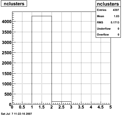
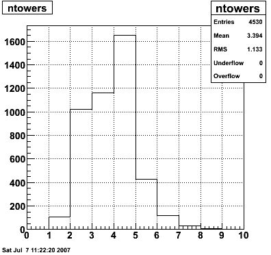
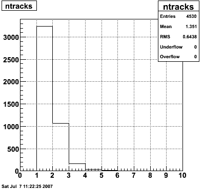
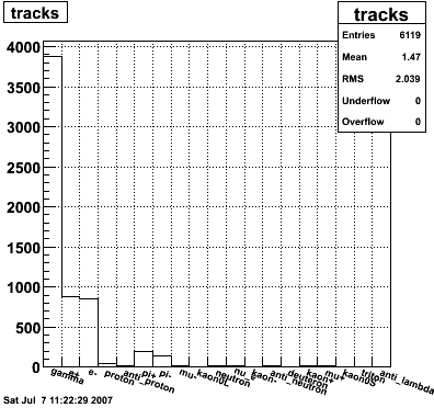
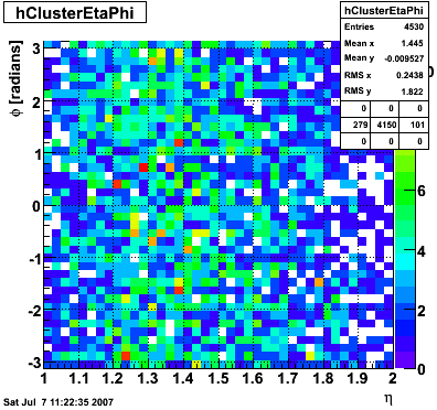
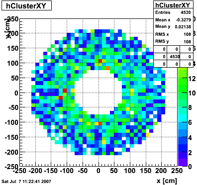
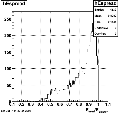
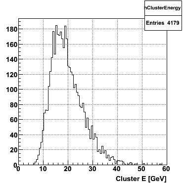
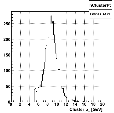
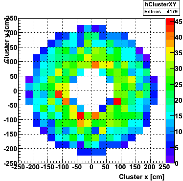
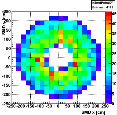
The plots below show the distribution of clusters in the endcap calorimeter for different partonic pT ranges. 2000 events were generated for each pT range. A cluster is made up of a central high tower above 3 GeV in pT and its surounding 8 neighbors. The total cluster pT must exceed 4.5 GeV.

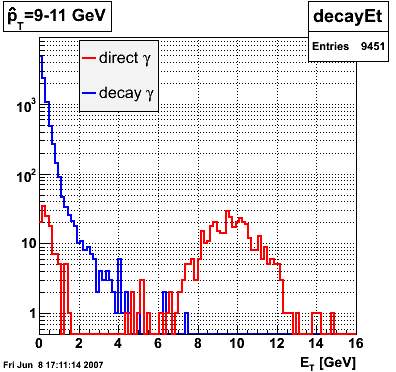
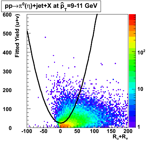
pT=9-11 GeV

Below is the pT of direct and decay photons from the Pythia record. Note how the two subsets are well separated at a given partonic pT. Any contamination to the direct photon signal would have to come from higher partonic pT.

Differences between Renee's and Manuel's Pythia records?

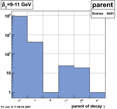
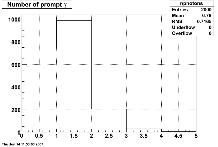
Number of prompt photons per event from GEANT record

Pibero Djawotho

Last updated Fri Jun 8 16:08:27 EDT 2007

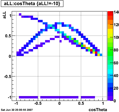
a_LL

Partonic a_LL

Jet	Gamma

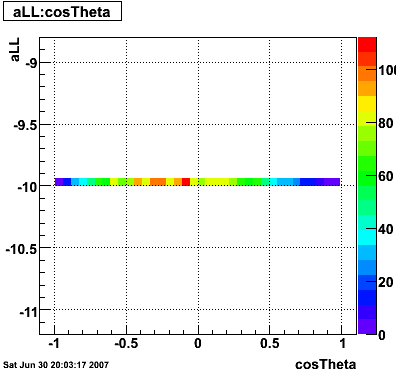Pibero Djawotho

Last updated Sat Jun 30 20:14:21 EDT 2007

gamma pT=9-11 GeV

Pibero Djawotho

Last modified Fri Jul 6 10:48:39 EDT 2007

gamma-jet kinematics

Clusters without parent track

Pibero Djawotho

Last updated Thu Jun 28 04:43:57 EDT 2007

gamma/X separation by energy

Pibero Djawotho

Last updated Wed Jul 11 11:10:26 EDT 2007

gamma/X separation by energy with pT weights

Pibero Djawotho

Last updated Thu Jul 12 00:28:35 EDT 2007

gamma/X separation by energy with pT weights and normalized by number of events

Pibero Djawotho

Last updated Wed Jul 18 14:55:08 EDT 2007

gamma/pi0 separation efficiency and rejection at pT=5-7 GeV

Pibero Djawotho

Last updated Wed Jul 4 17:45:26 EDT 2007

gamma/pi0 separation efficiency and rejection at pT=9-11 GeV

Pibero Djawotho

Last updated Wed Jul 4 13:23:41 EDT 2007

gamma/pi0 separation efficiency and rejection at pT=9-11 GeV

Pibero Djawotho

Last updated Wed Jul 4 13:23:41 EDT 2007

2007.07.09 How to run the gamma fitter

How to run the gamma fitter

The gamma fitter runs out of the box. The code consists of the classes StGammaFitter and StGammaFitterResult in CVS. After checking out a copy of offline/StGammaMaker, cd into the offline directory and run:

root4star StRoot/StGammaMaker/macros/RunGammaFitterDemo.C

The following plots will be generated on the ROOT canvas and dumped into PNG files.

Pibero Djawotho

Last modified Mon Jul 9 18:40:07 EDT 2007

2007.07.25 Revised gamma/pi0 algorithm in 2006 p+p collisions at sqrt(s)=200 GeV

Revised gamma/pi0 algorithm in 2006 p+p collisions at sqrt(s)=200 GeV

Description

The class

StGammaFitter

computes the maximal sided residual of the SMD response in the u- and v-plane for gamma candidates. It is based on C++ code developed by Jason Webb from the original code by Les Bland who got the idea from CDF (?) The algorithm follows the steps below:

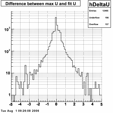
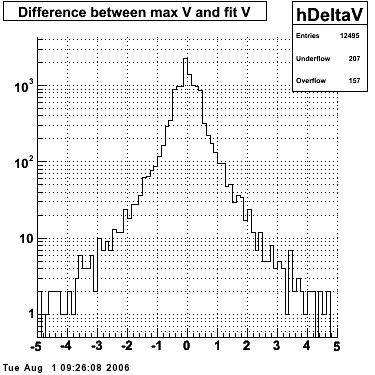
The SMD response, which is SMD strips with hits in MeV, in each plane (U and V) is stored in histogram hU and hV.
Fit functions fU and fV are created. The functional form of the SMD peak is a double-Gaussian with common mean and fixed widths. The widths were obtained by the SMD response of single photons from the EEMC slow simulator. As such, the only free parameters are the common mean and the total yield. The actual formula used is: [0]*(0.69*exp(-0.5*((x-[1])/0.87)**2)/(sqrt(2*pi)*0.87)+0.31*exp(-0.5*((x-[1])/3.3)**2)/(sqrt(2*pi)*3.3))
- [0] = yield
- [1] = mean
The mean is fixed to the strip with maximum energy and the yield is adjusted so the height of the fit matches that of the mean.
The residual for each side of the peak is calculated by subtracting the fit from the data (residual = data - fit) from 2 strips beyond the mean out to 40 strips.
The maximal sided residual is the greater residual of each side.

Code

Candidates selection

2006 p+p at 200 GeV dataset from Sivers analysis (from Jan Balewski)
/star/institutions/iucf/balewski/prodOfficial06_muDst/
Gamma candidate from gamma maker: 3x3 clusters with pt > 5 GeV
No track pointing to cluster
Minimum of 3 SMD hits in each plane
Cuts from Jan & Naresh electron analysis:
- Preshower 1 energy > 0.5 MeV
- Preshower 2 energy > 2.0 MeV
- Postshower energy < 0.5 MeV
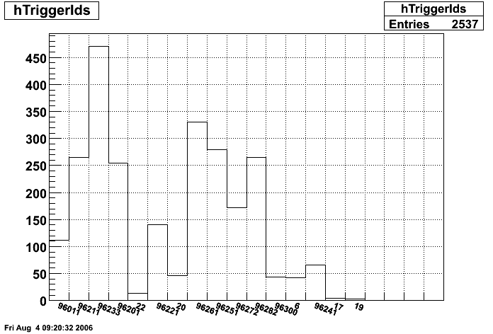
The triggers caption in the PDF files shows the trigger id's satisfied by the event. A red trigger id is a L2-gamma trigger. I observe that generally the L2-gamma triggered event are a bit cleaner. Also shown is the pt and energy of the cluster.

Raw SMD response

The parameters of the isolation cut were suggested by Steve Vigor:

Hi Pibero,

  In general, I believe people have used smaller cone radii for isolation
cuts than for jet reconstruction (where the emphasis is on trying to
recover full jet energy).  So you might try something like requiring
that no more than 10 or 20% of the candidate cluster E_T appears
in scalar sum p_T for tracks and towers within a cone radius of
0.3 surrounding the gamma candidate centroid, excluding the
considered cluster energy.  The cluster may already contain energy
from other jet fragments, but that should be within the purview of
the gamma/pi0 discrimination algo to sort out.  For comparison, Les
used a cone radius of 0.26 for isolation cuts in his original simulations
of gamma/pi0 discrimination with the endcap.  Using much larger
cone radii may lead to accidental removal of too many valid gammas.


Steve

Pibero Djawotho

Last updated Wed Jul 25 10:07:07 EDT 2007

2007.09.12 Endcap Electrons

Endcap Electrons

This analysis is based on the work of Jan and Justin on SMD Profile Analysis for different TPC momenta. See here for a list of cuts. The original code used by Jan and Justin is here.

Transverse running

Analysis uses 64 out of 300 runs from 2006 pp transverse run

MuDst are located at:

/star/institutions/iucf/balewski/prodOfficial06_muDst/

No trigger selection

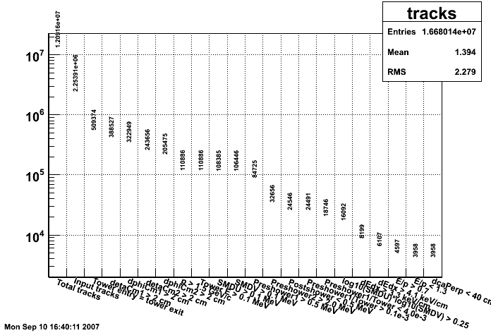
Figure 1: Number of tracks surviving each successive cut

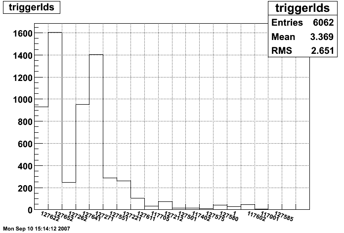
Figure 2a: Number of tracks per trigger id for all electron candidates. Most common trigger ids are:

127652	eemc-jp0-etot-mb-L2jet	EEMC JP > th0 (32, 4 GeV) and ETOT > TH (109, 14 GeV), minbias condition, L2 Jet algorithm, reading out slow detectors, transverse running
127271	eemc-jp1-mb	EEMC JP > th1 (49, 8 GeV) && mb, reading out slow detectors, transverse running
127641	eemc-http-mb-l2gamma	EEMC HT > th1 (12, 2.6 GeV, run < 7100052;13, 2.8 GeV, run >=7100052) and TP > TH1 (17, 3.8 GeV, run < 710052; 21, 4.7 GeV, run>=7100052 ), minbias condition, L2 Gamma algorithm, reading out slow detectors, L2 thresholds at 3.4, 5.4, transverse running
127622	bemc-jp0-etot-mb-L2jet	BEMC JP > th0 (42, 4 GeV) and ETOT > TH (109, 14 GeV), minbias condition, L2 Jet algorithm, reading out slow detectors, transverse running; L2jet thresholds at 8.0,3.6,3.3

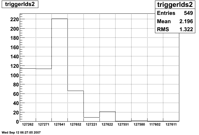
Figure 2b: Number of tracks per trigger id for all electron candidates for p_T > 4 GeV. The dominant trigger ids become:

127641	eemc-http-mb-l2gamma	EEMC HT > th1 (12, 2.6 GeV, run < 7100052;13, 2.8 GeV, run >=7100052) and TP > TH1 (17, 3.8 GeV, run < 710052; 21, 4.7 GeV, run>=7100052 ), minbias condition, L2 Gamma algorithm, reading out slow detectors, L2 thresholds at 3.4, 5.4, transverse running
127262	eemc-ht2-mb-emul	EEMC HT > th2 (22, 5.0 GeV) && mb, reading out slow detectors, emulated in L2, transverse running, different threshold from 117262
127271	eemc-jp1-mb	EEMC JP > th1 (49, 8 GeV) && mb, reading out slow detectors, transverse running
127652	eemc-jp0-etot-mb-L2jet	EEMC JP > th0 (32, 4 GeV) and ETOT > TH (109, 14 GeV), minbias condition, L2 Jet algorithm, reading out slow detectors, transverse running

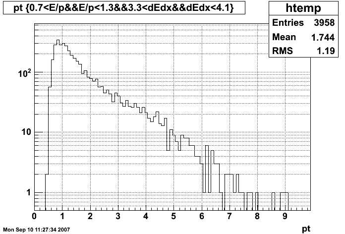
Figure 3: p_T distribution of tracks before E/p, dE/dx and pT cut

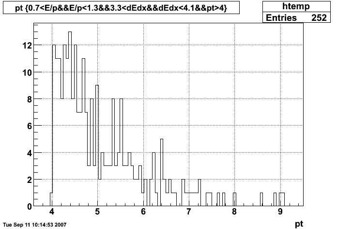
Figure 4: p_T distribution of electron candidates with p_T > 4 GeV

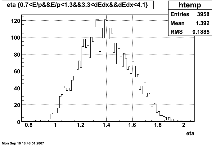
Figure 5: η distribution of electron candidates (all p_T)

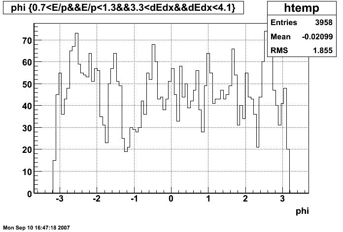
Figure 6: φ distribution of electron candidates (all p_T)

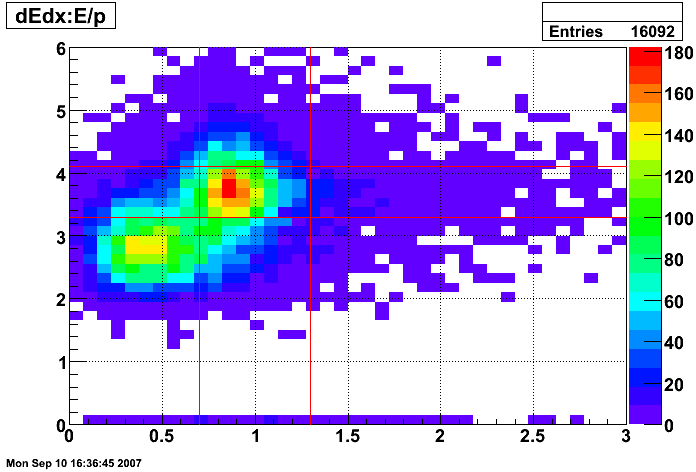
Figure 7: dE/dx of tracks before E/p and dE/dx cuts (all p_T)

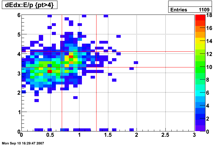
Figure 8: dE/dx of tracks before E/p and dE/dx cuts (p_T > 4 GeV)

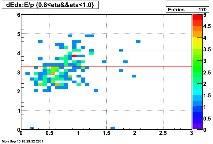
Figure 9: dE/dx of tracks before E/p and dE/dx cuts (all p_T and 0.8 < η < 1.0)

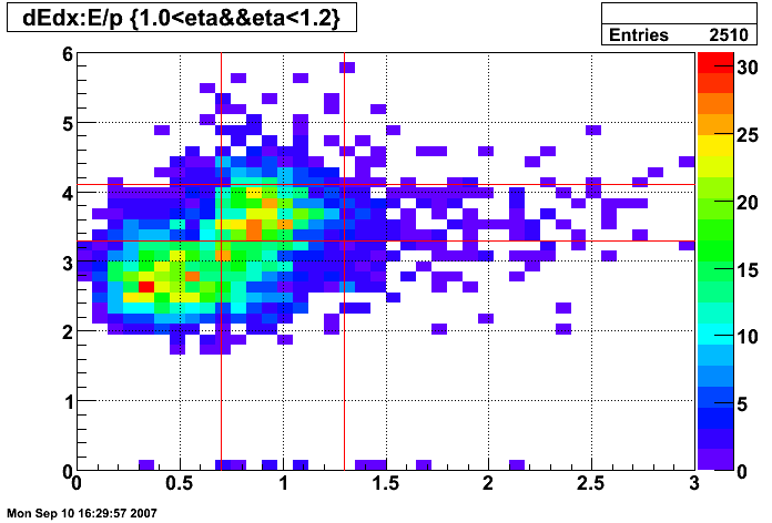
Figure 10: dE/dx of tracks before E/p and dE/dx cuts (all p_T and 1.0 < η < 1.2)

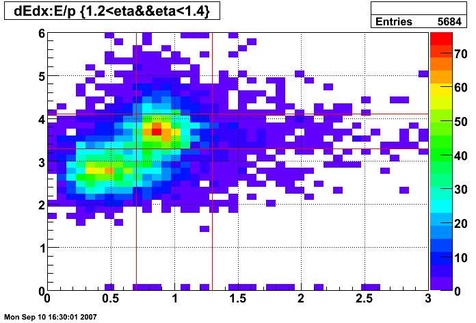
Figure 11: dE/dx of tracks before E/p and dE/dx cuts (all p_T and 1.2 < η < 1.4)

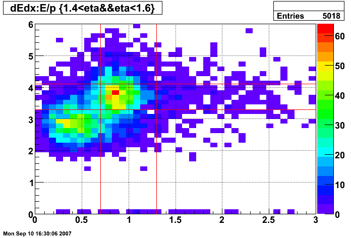
Figure 12: dE/dx of tracks before E/p and dE/dx cuts (all p_T and 1.4 < η < 1.6)

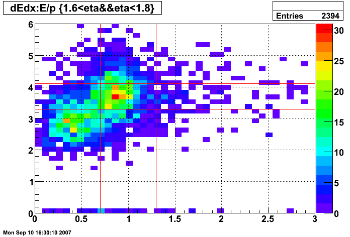
Figure 13: dE/dx of tracks before E/p and dE/dx cuts (all p_T and 1.6 < η < 1.8)

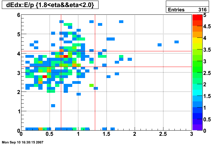
Figure 14: dE/dx of tracks before E/p and dE/dx cuts (all p_T and 1.8 < η < 2.0)

Click here for SMD profiles of transverse electron candidates.
Click here for ROOT file with transverse electrons ntuple.

Longitudinal running

MuDst are located at:

/star/institutions/iucf/hew/2006ppLongRuns/

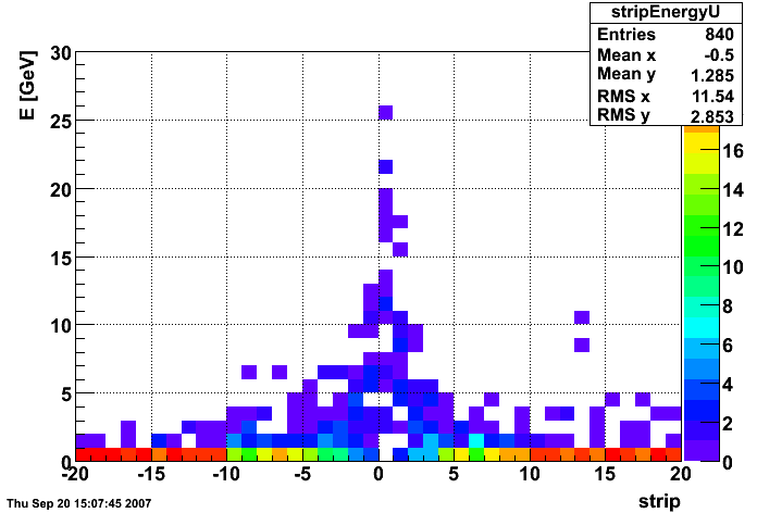
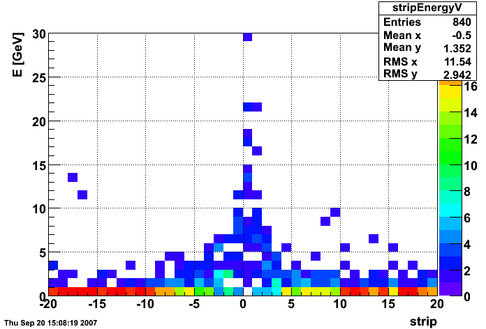
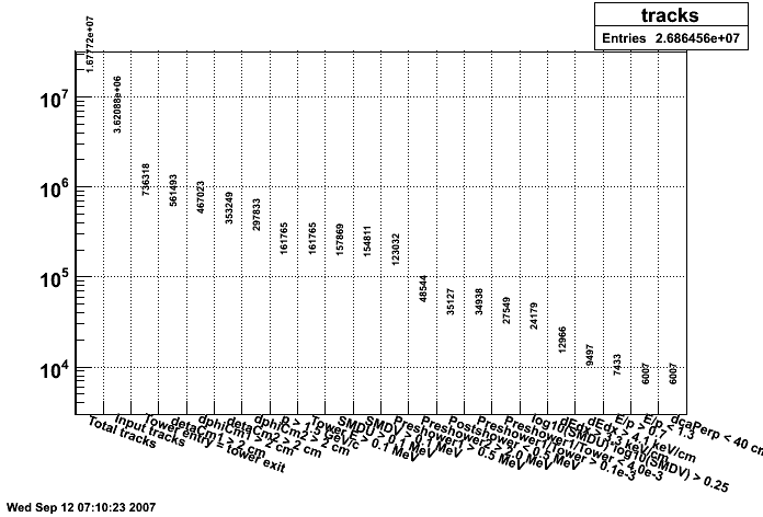
Figure 2.1

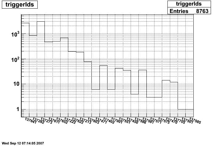
Figure 2.2: The dominant trigger ids are:

137273	eemc-jp1-mb	EEMC JP > th1 (52, 8.7 GeV) && mb, reading out slow detectors, longitudinal running 2
137641	eemc-http-mb-l2gamma	EEMC HT > th1 (16, 3.5 GeV) and TP > th1 (20, 4.5 GeV), minbias condition, L2 Gamma algorithm, reading out slow detectors, L2 thresholds at 3.7, 5.2, longitudinal running 2
137262	eemc-ht2-mb-emul	EEMC HT > th2 (22, 5.0 GeV) && mb, reading out slow detectors, emulated in L2, longitudinal running 2
137222	bemc-jp1-mb	BEMC JP > th1 (60, 8.3 GeV) && mb, reading out slow detectors, longitudinal running 2

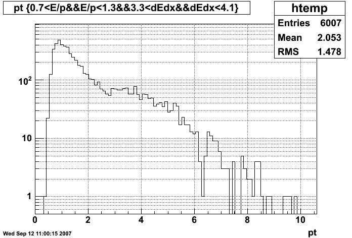
Figure 2.3a

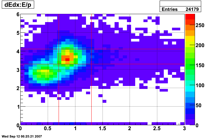
Figure 2.3

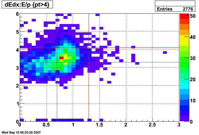
Figure 2.4

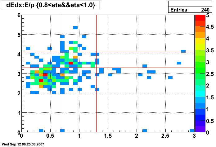
Figure 2.5

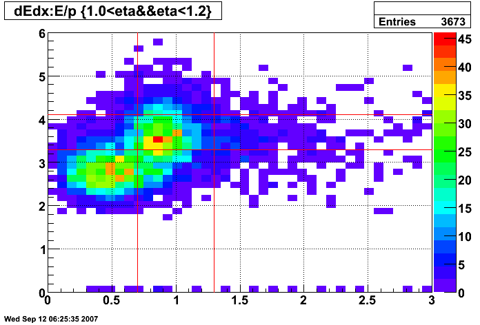
Figure 2.6

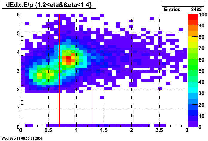
Figure 2.7

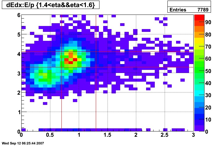
Figure 2.8

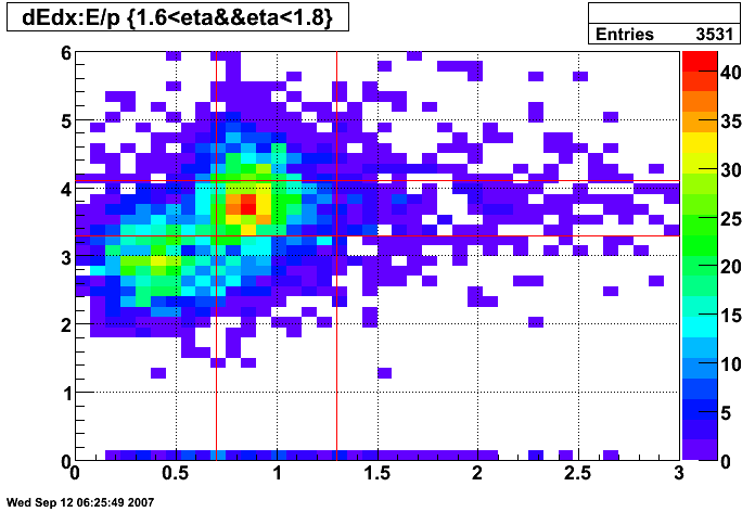
Figure 2.9

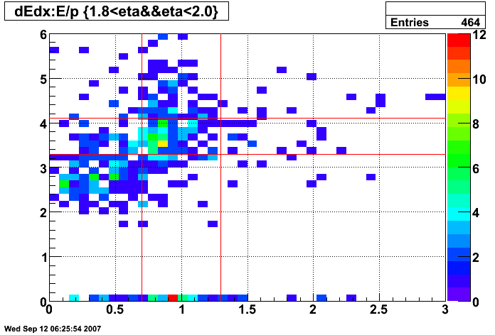
Figure 2.10

Click here for SMD profiles of longitudinal electron candidates.
Click here for ROOT file with longitudinal electrons ntuple.

Code

Click here for a tarball of the code used in this analysis.

Summed SMD response

SMD response function

f(x)=p0*(0.69*exp(-0.5*((x-p1)/0.87)**2)/(sqrt(2*pi)*0.87)+0.31*exp(-0.5*((x-p1)/3.3)**2)/(sqrt(2*pi)*3.3))

```
p0 = yield
```
```
p1 = centroid
```

Transverse

21 electrons

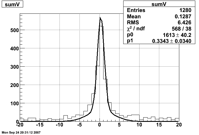
Longitudinal

99 electrons

Pibero Djawotho

Last updated Wed Sep 12 08:29:53 EDT 2007

2008.01.23 Endcap etas

Endcap etas

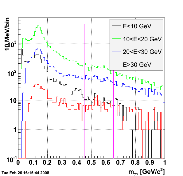
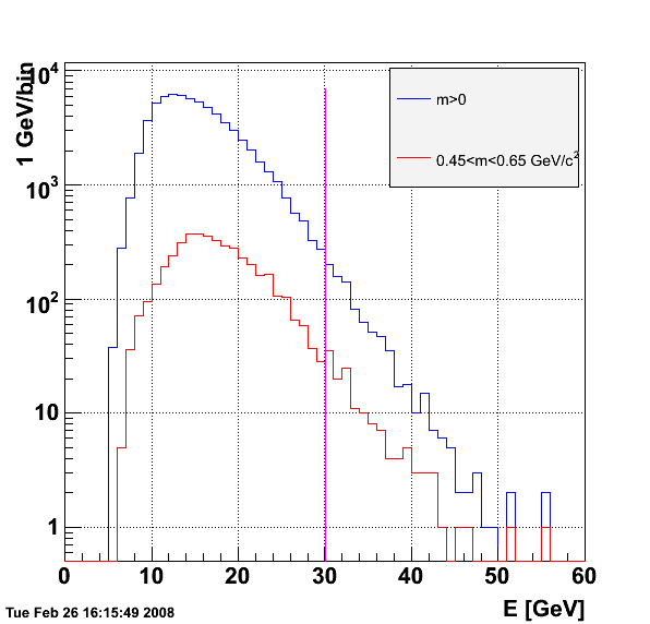
This analysis to look for etas at higher energy is in part motivated by this study. The interest in etas, of course, is that their decay photons are well separated at moderate energies (certainly more separated than the photons from pi0 decay). I ran Weihong's pi0 finder with tower seed threshold of 0.8 GeV and SMD seed threshold of 5 MeV (I believe his default SMD seed setting is 2 MeV). I then look in the 2-photon invariant mass region between 0.45 and 0.65 GeV (the PDG nominal mass for the eta is 0.54745 +/- 0.00019 GeV). I observe what looks like a faint eta peak. The dataset processed is the longitudinal 2 run of 2006 from the 20 runs sitting on the IUCF disk in Weihong's directory (/star/institutions/iucf/hew/2006ppLongRuns/).

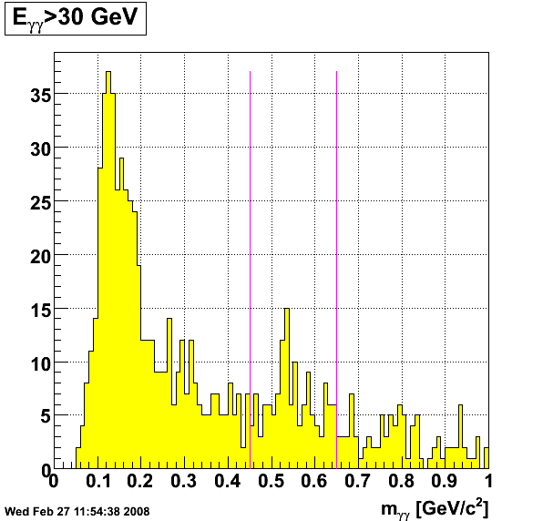
Within the reconstructed mass window 0.45 to 0.65 GeV, I take a look at the decay photon shower profiles in the SMD. The samples are saved in the file etas.pdf. For the most part, these shower shapes are cleaner than the original sample. Although the statistics are not great.

Additional Material

Documents

Pibero Djawotho

Last updated Wed Jan 23 12:35:43 EST 2008

2008.02.27 ESMD shape library

ESMD shape library

Shower Widths for Monte Carlo and Data

Description

Hal did a comparison of the widths of the shower shapes between Monte Carlo and data. Below is a description of what was done.

      I took the nominal central value, either from the maxHit or the
nominal central value, and added the energy in the +/- 12 strips.  Then I
computed the mean strip (which may have been different from the nominal
central value!!).  I normalized the shape to give unit area for each smd
cluster, and added to the histograms separately for U and V and for MC and
data (= Will's events).  I did NOT handle Will's events correctly, just
using whatever event was chosen randomly, rather than going through his
list sequentially.  Note I ran 1000 events, and got 94 events in my shower
shape histos.

      So, there are several minor problems.  1) I didn't go through Will's
events sequentially.  2) I normalized, but perhaps not to the correct 25
strips, because the mean strip and the nominal strip may have differed.
3) there may have been a cutoff on some events due to being close to one
end of the smd plane (near strip 0 or 287).  My sense from looking at the
plots is that these don't matter much.

      The conclusion is that the MC shape is significantly narrower than
the shape from Will's events, which is obviously narrower than the random
clusters we were using at first with no selection for the etas.  Hence, we
are not wasting our time with this project.

Decsription of Pythia Sample

A few histograms were added to the code:

MC is Pythia gamma-jet at partonic pT 9-11 GeV with gamma in the Endcap
Data is from Will Jacobs golden events from Weihong sample
Require no conversion
Require all hits from direct photon in same sector

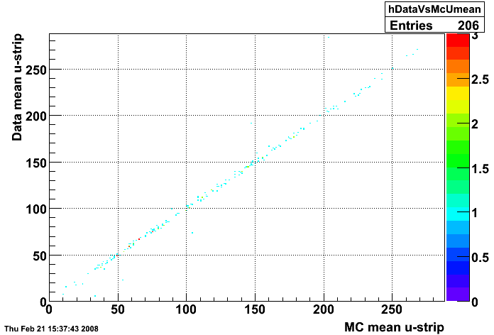
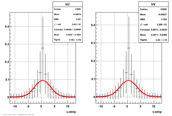
Figure 1:

Data vs. MC mean u-strip

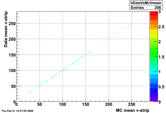
Figure 2:

Data vs. MC mean v-strip

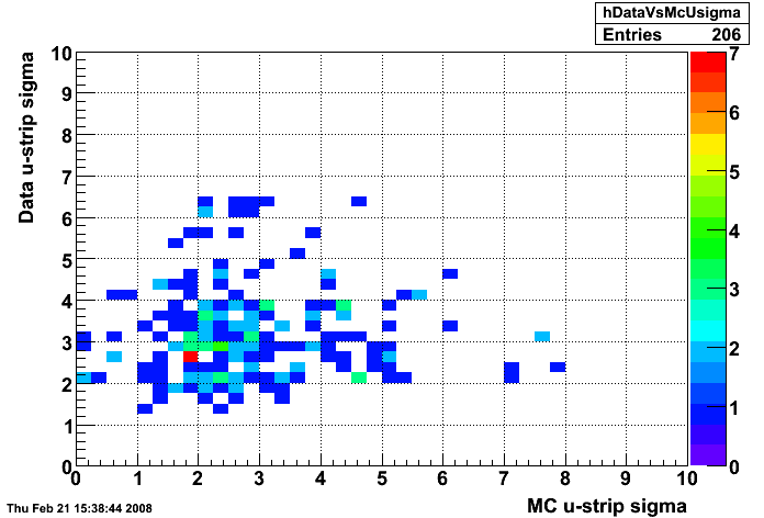
Figure 3:

Data vs. MC u-strip sigma

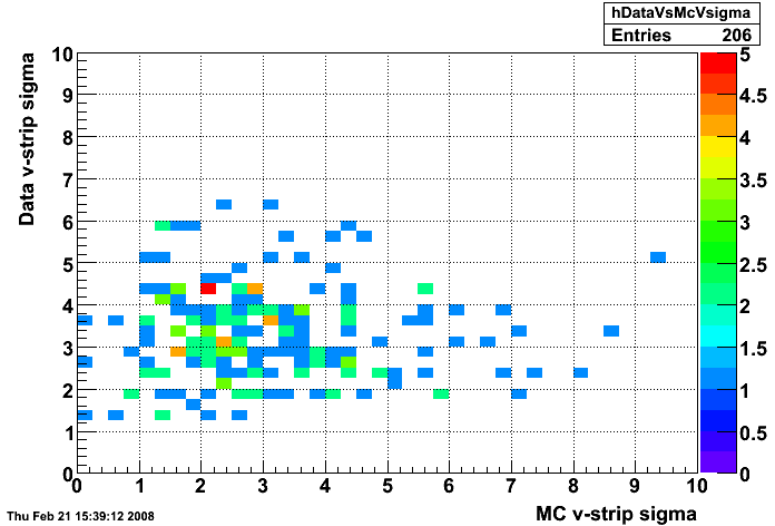
Figure 4:

Data vs. MC v-strip sigma

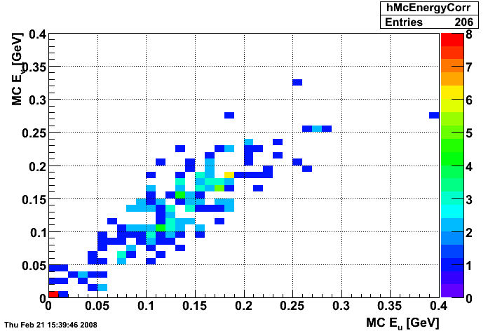
Figure 5:

MC E

_v

vs. E

_u

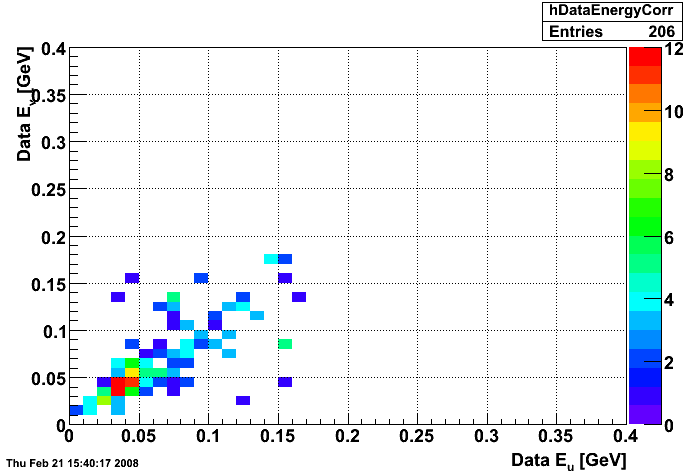
Figure 6:

Data E

_v

vs. E

_u

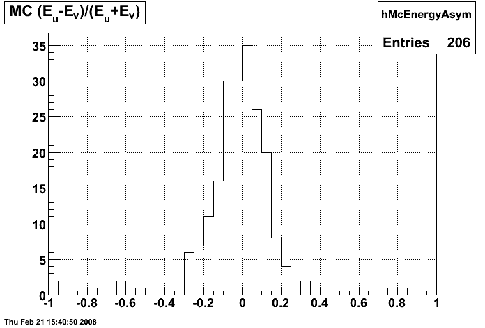
Figure 7:

MC energy asymmetry in SMD planes

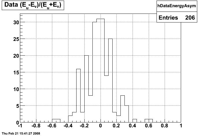
Figure 8:

Data energy asymmetry in SMD planes

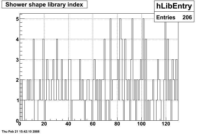
Figure 9:

Shower shape library index used (picked at random)

Single events shower shapes are displayed in

esmd.pdf

or

esmd_solid.pdf

.

green = projected position of direct photon in the Endcap
blue = Monte Carlo SMD response
red = Data SMD response

Hal Spinka

Pibero Djawotho

Last modified Wed Feb 27 09:51:27 EST 2008

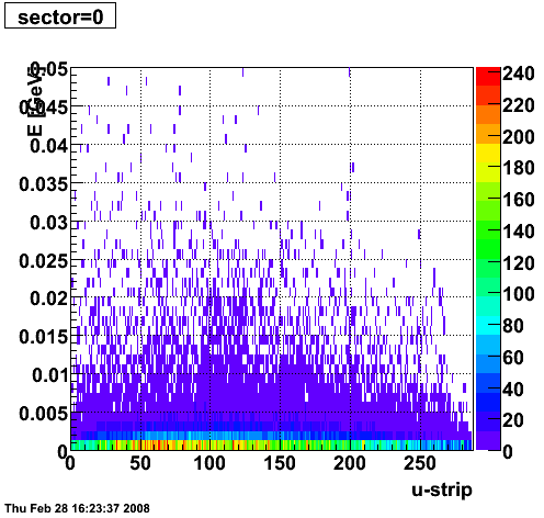
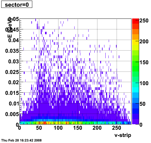
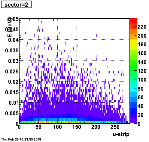
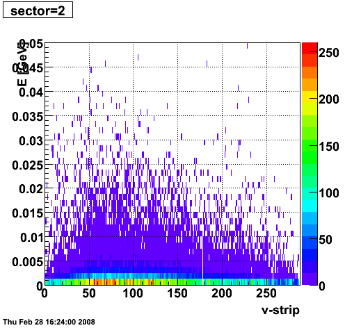
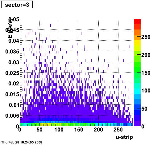
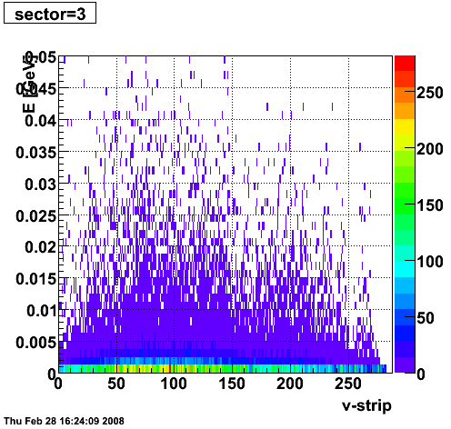
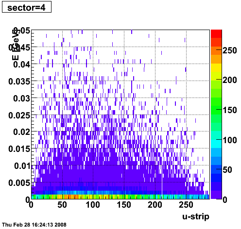
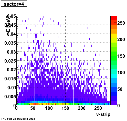
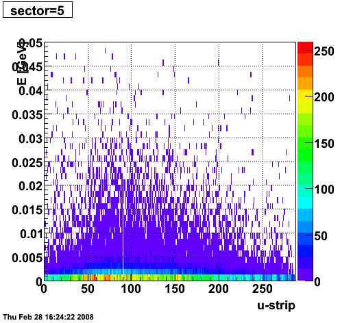
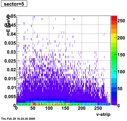
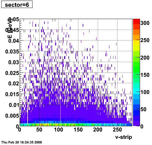
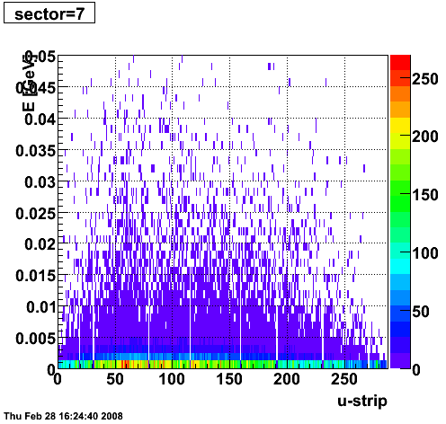
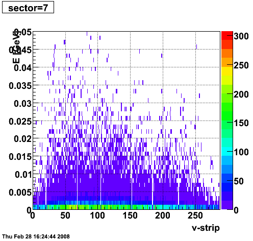
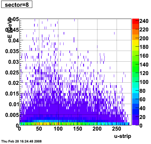
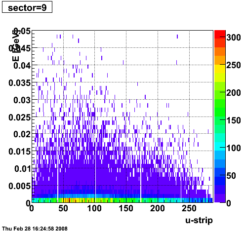
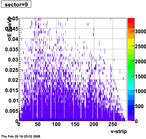
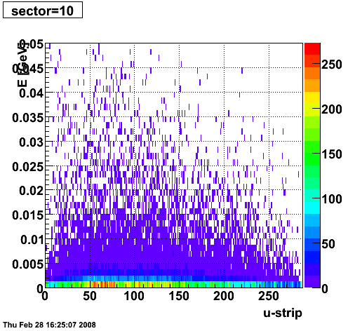
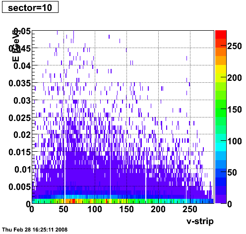
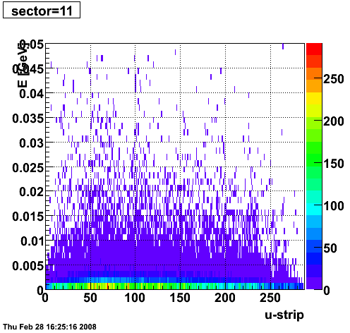
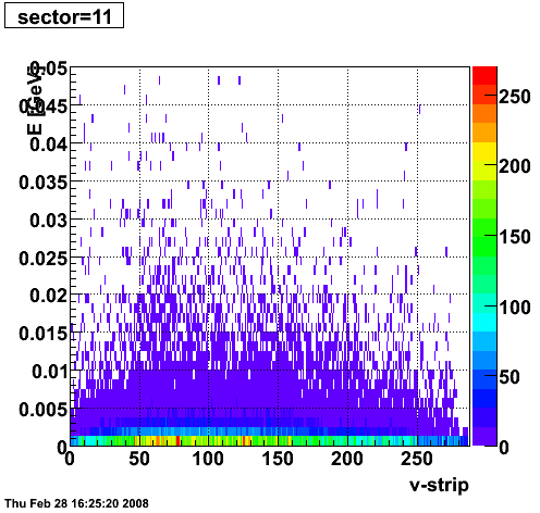
2008.02.28 ESMD QA for run 7136033

ESMD QA for run 7136033

Pibero Djawotho

Last updated Thu Feb 28 16:17:55 EST 2008

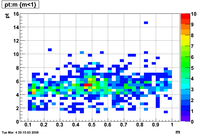
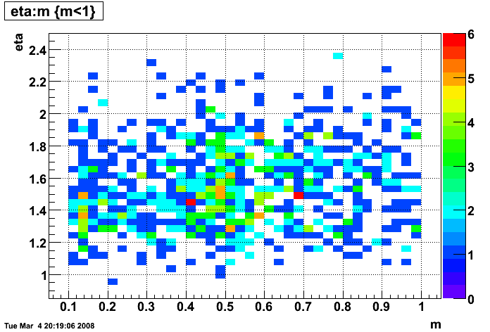
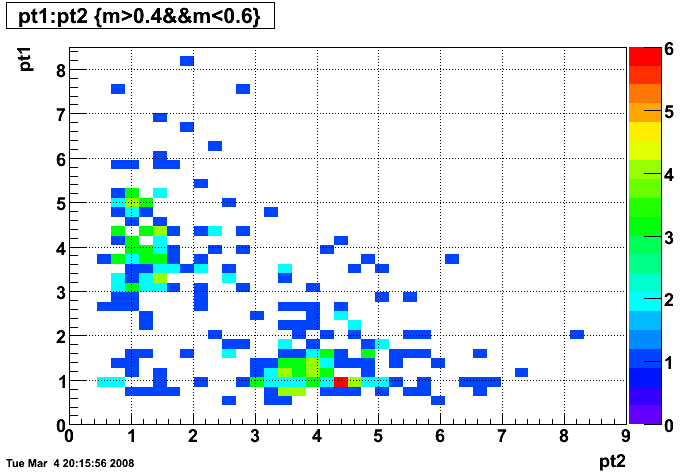
2008.03.04 A second look at eta mesons in the STAR Endcap Calorimeter

A second look at eta mesons in the STAR Endcap Calorimeter

Introduction

In case you missed it, the first look is

here

. I processed

44 runs

from the 2006 pp longitudinal 2 runs and picked events tagged with the L2gamma trigger id (137641). I ran the StGammaMaker on the MuDst files from these runs and produced gamma trees. These gamma trees are available at

/star/institutions/iucf/pibero/2007/etaLong/

. Within the StGammaMaker framework, I developed code to seek candidate etas with emphasis on high purity. The macros and source files are:

Note, the workhorse function is

StEtaFinder::findTowerPoints()

.

Algorithm

Find seed tower with pT > 0.8 GeV
Require no TPC track into the seed tower
Get the ranges of SMD U & V strips that span the volume of the seed tower
Find the strips with maximum energy within these ranges
Require that the maximum strips have more than 2 MeV in each SMD plane
Get the intersection of the maximum strips and ensures that it lies within 70% of the fiducial volume of the seed tower
Make sure the photon candidate responsible for the SMD clusters above enters and exits the same seed tower
Form a 11-strip cluster in each plane with +/-5 strips around the max strip and require that it contains 70% of the energy in a range +/-20 strips around the max strip
Require that the energy asymmetry between the 11-strip clusters in the U and V planes be less than 20%
Create a point using the energy of the seed tower and the position of the intersection of the max strips in the SMD U and V planes
Repeat until seed towers in the event are exhausted
Combine different points in the event to calculate the invariant mass
Diphoton pairs with invariant mass between 0.4 and 0.6 GeV are saved to a PDF file

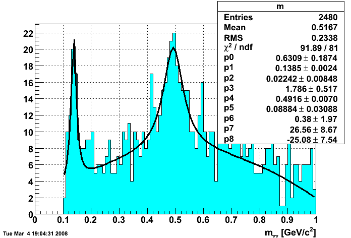
Invariant mass

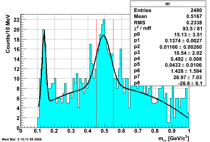
I fit the diphoton invariant mass with two Gaussians, one for the pi0 peak (p0-p2) and another one for the eta peak (p3-p5) plus a quadratic for the background (p6-p8). The Gaussian is of the form p0*exp(0.5*((x-p1)/p2)**2) and the quadratic is of the form p6*+p7*x+p8*x**2. A slightly better chi2/ndf in the fit is achieved by using Breit-Wigner functions instead of Gaussians for the signal here. I calculate the raw yield of etas from the fit as p3*sqrt(2*pi)*p5/bin_width = 85 where each bin is 0.010 GeV wide. I select candidate etas in the mass range 0.45 to 0.55 GeV and plot their photon response in the shower maximum detector here. Since we are interested in collecting photons of pT > 7 GeV, only those candidate photons with pT > 5 GeV will be used in the shower shape library. I also calculate the background under the signal region by integrating the background fit from 0.45 to 0.55 GeV and get 82 counts.

S = 85
B = 82
S:B = 1.03:1
S/√S+B = 6.6

Additional plots

PhotonsFromEtas.txt
PhotonsFromEtas2.txt

Pibero Djawotho

Last updated at Tue Mar 4 16:21:13 EST 2008

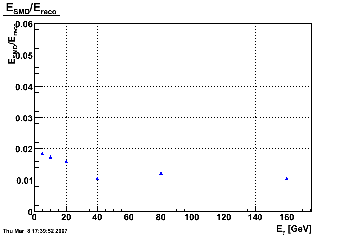
2008.03.08 Adding the SMD energy to E_reco/E_MC for Photons

Adding the SMD energy to E_reco/E_MC for Photons

The following is a revisited study of E_reco/E_MC for photons with the addition of the SMD energy to E_reco.

QA plots for each energy

E_SMD/E_reco vs. eta

Pibero Djawotho

Last updated Thu Mar 8 04:27:28 EST 2007

2008.03.21 Chi square method

Chi square method

 SectorVsRunNumber.png   10-Feb-2010 12:22   14K  
 ShowerShapes.png        10-Feb-2010 12:22   17K  
 chiSquareMC.png         10-Feb-2010 12:22   13K  
 chiSquarePibero.png     10-Feb-2010 12:22   16K  
 chiSquareWill.png       10-Feb-2010 12:22   16K  
 chiSquareWillAndMC.png  10-Feb-2010 12:22   17K

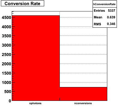
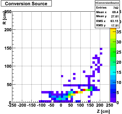
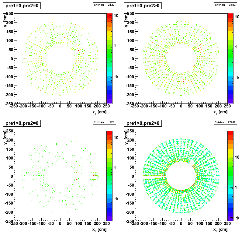
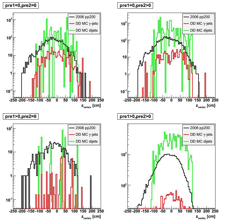
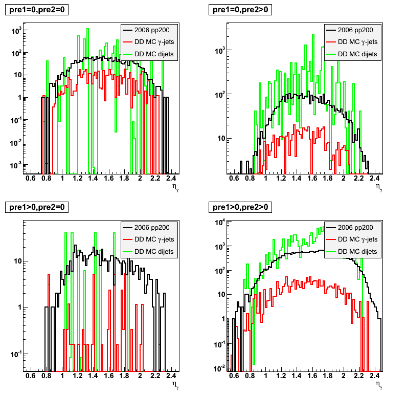
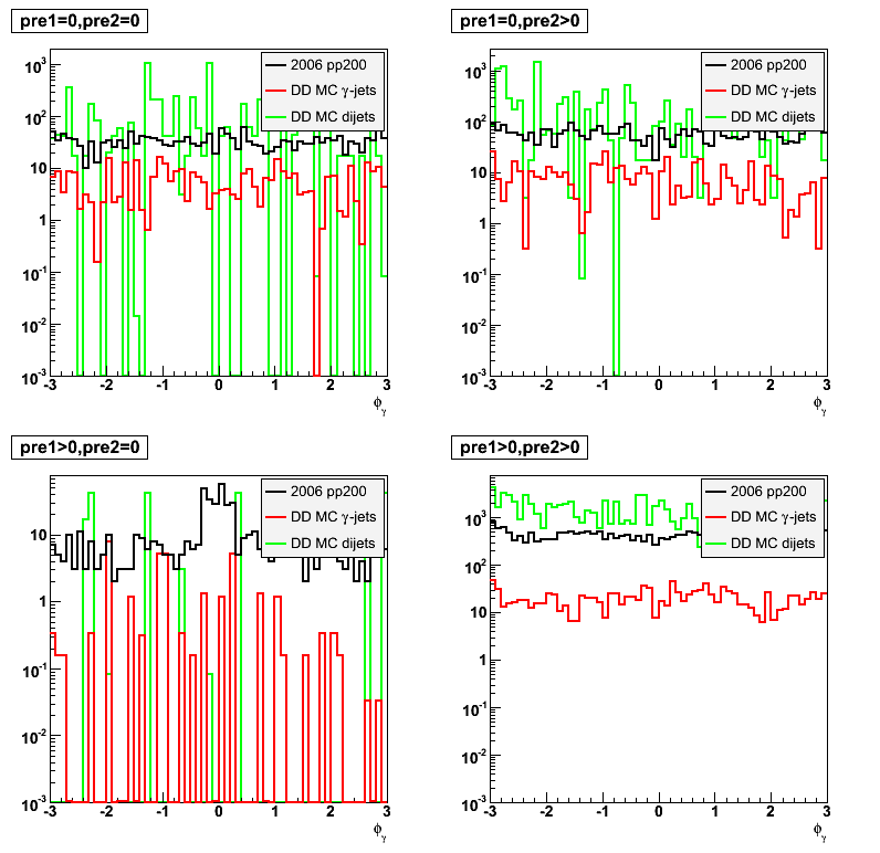
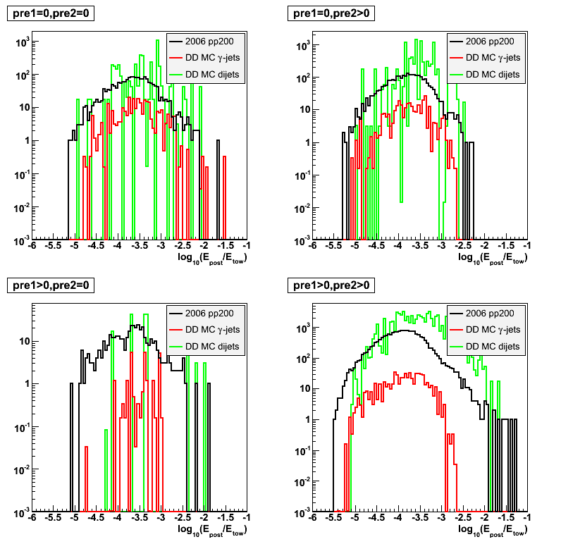
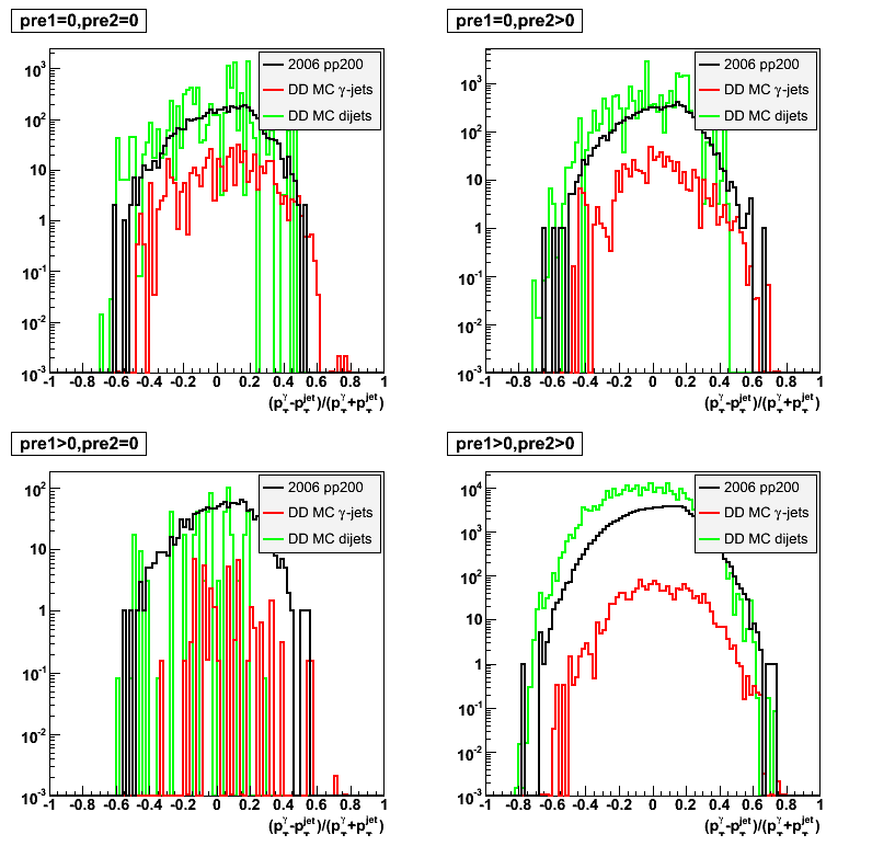
2008.04.08 Data-Driven Shower Shapes

Data-Driven Shower Shapes

Gamma Conversion before the Endcap

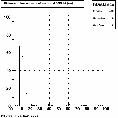
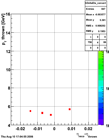
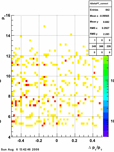
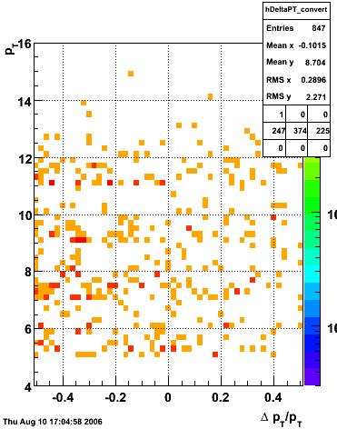
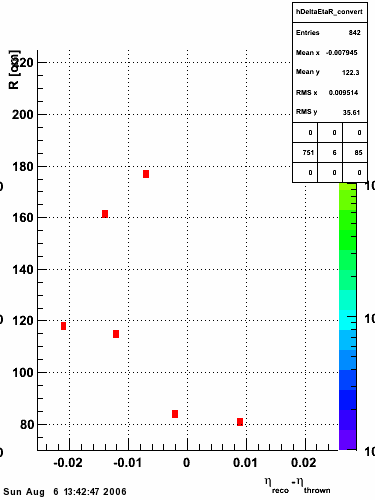
The plots below show the conversion process before the Endcap. I look at prompt photons heading towards the Endcap from a MC gamma-jet sample with a partonic pT of 9-11 GeV. I identify those photons that convert using the GEANT record. The top left plot shows the total number of direct photons and those that convert. I register a 16% conversion rate. This is consistent with Jason's 2006 SVT review. The top right plot shows the source of conversion, where most of the conversions emanate from the SVT support cone, also consistent with Jason's study. The bottom left plot shows the separation in the SMD between the projected location of the photon and the location of the electron/positron from conversion.

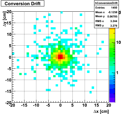Shower shapes comparison

This

PDF

file shows several shower shapes in a single plot for comparison:

MC - Monte Carlo shower shape from the 9-11 GeV pT gamma-jet Pythia sample
DD - Data-driven Monte Carlo shower shape (Each final state photon shower shape is replaced with a corresponding shower shape from data in the same sector configuration, energy, preshower, and U/V-plane bin).
Standard MC - Monte Carlo shower shape parametrized by Hal (also from the 9-11 GeV pT gamma-jet Pythia sample)
Will - Data shower shape derived from photons from eta decays by Will using a modified version of Weihong/Jason meson pi0 finder
Pibero - Data shower shape derived from photons from eta decays by Pibero using a crude eta finder

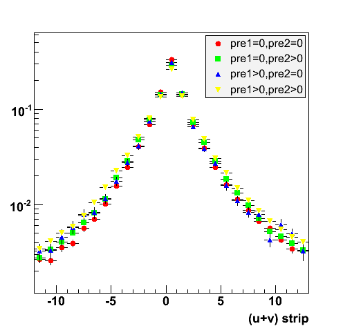
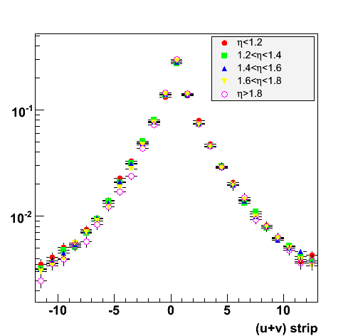
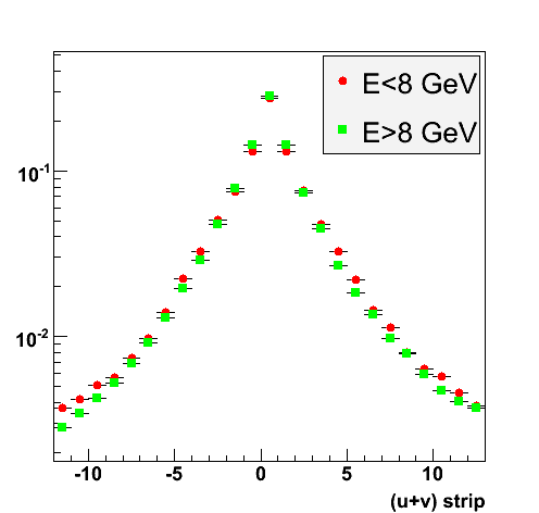
Shower Shapes Sorted by SMD Plane, Sector Configuration, Energy and Preshower

These Shower Shapes are binned by:

SMD plane (U and V)
Sector configuration with the formula sector%3 where sector=1..12, so 3 different bins. More details can be found at the EEMC Web site under the Geometry link.
Energy of the photon (E < 8 GeV and E > 8 GeV)
Preshower energy (pre1==0&&pre2==0) and (pre1>0||pre2>0)

They are then fitted with a triple-Gaussian of the form:

[0]*([2]*exp(-0.5*((x-[1])/[3])**2)/(sqrt(2*pi)*[3])+[4]*exp(-0.5*((x-[1])/[5])**2)/(sqrt(2*pi)*[5])+(1-[2]-[4])*exp(-0.5*((x-[1])/[6])**2)/(sqrt(2*pi)*[6]))

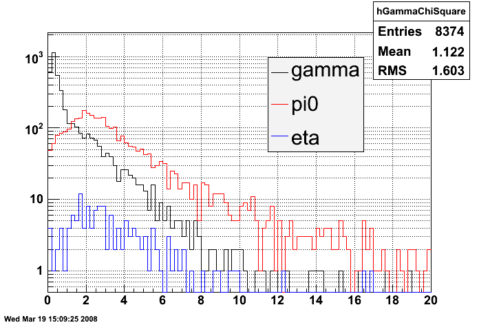
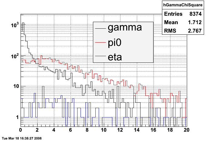
Comparison of Sided Residuals for Monte Carlo (MC) and Data-Driven (DD) Shower Shapes

All fits to MC are with reference to the old Monte carlo fit function:

[0]*(0.69*exp(-0.5*((x-[1])/0.87)**2)/(sqrt(2*pi)*0.87)+0.31*exp(-0.5*((x-[1])/3.3)**2)/(sqrt(2*pi)*3.3))

All fits to the data are with reference to a single

Shower Shape

. The fit function is:

[0]*([2]*exp(-0.5*((x-[1])/[3])**2)/(sqrt(2*pi)*[3])+[4]*exp(-0.5*((x-[1])/[5])**2)/(sqrt(2*pi)*[5])+(1-[2]-[4])*exp(-0.5*((x-[1])/[6])**2)/(sqrt(2*pi)*[6]))

Comparison of Sided Raw Tails for Monte Carlo (MC) and Data-Driven (DD) Shower Shapes

Pibero Djawotho

Last updated Tue Apr 8 17:29:40 EDT 2008

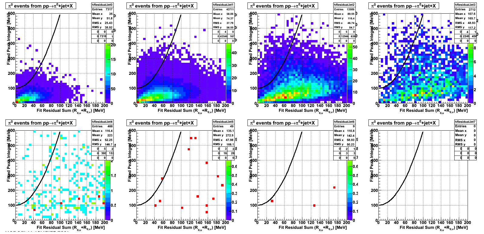
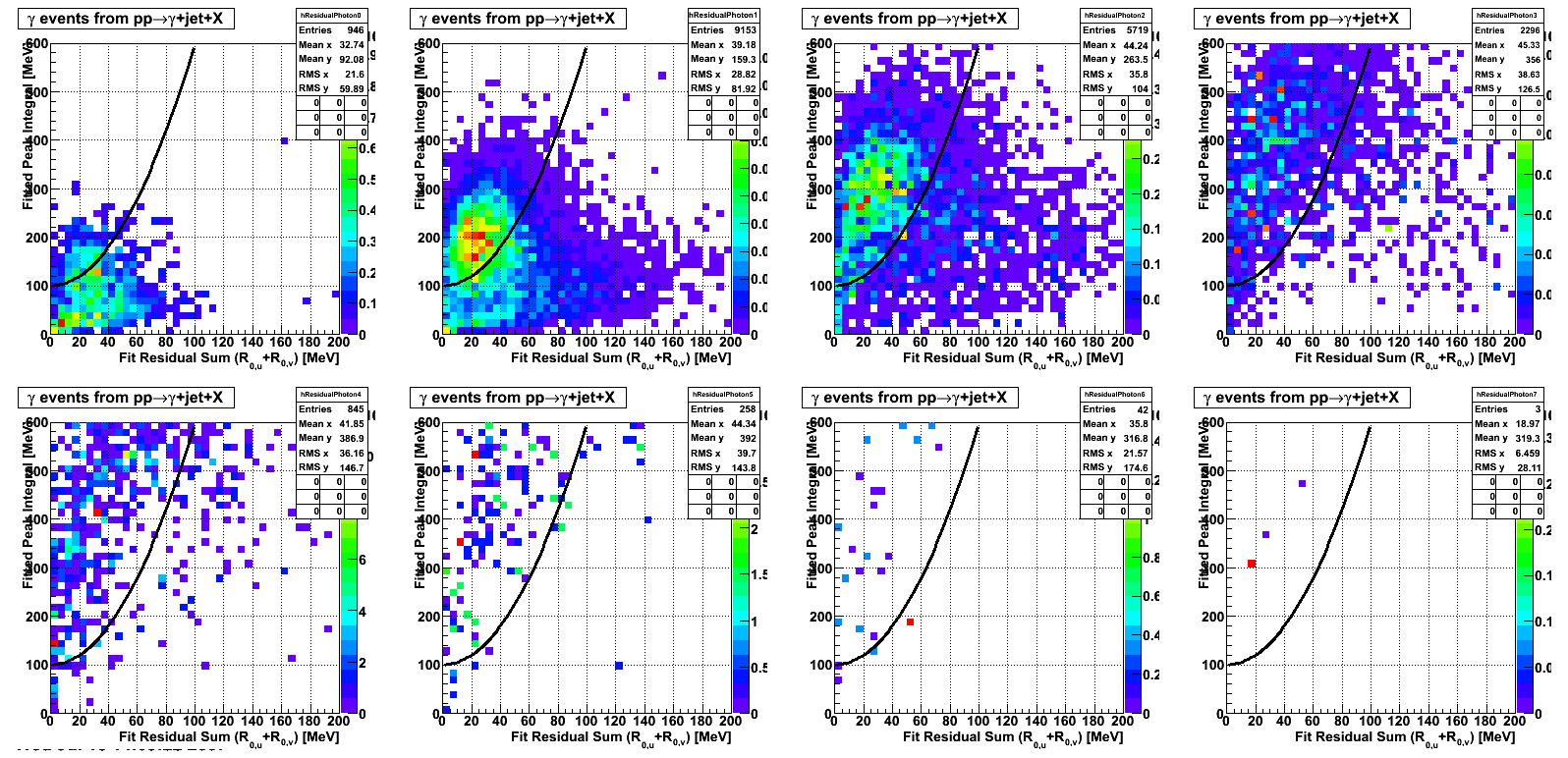
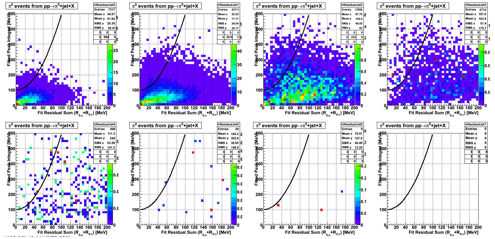
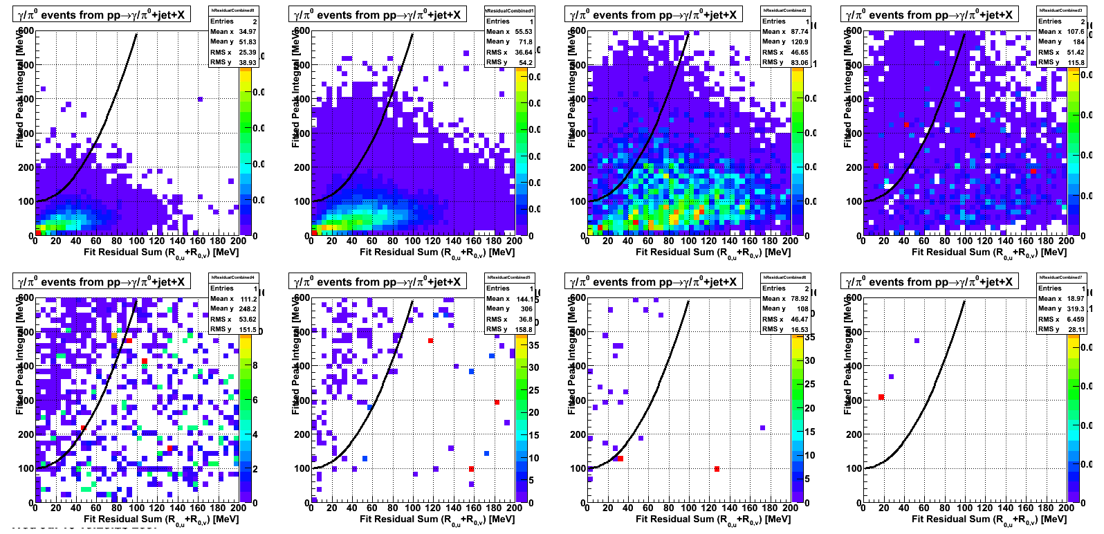
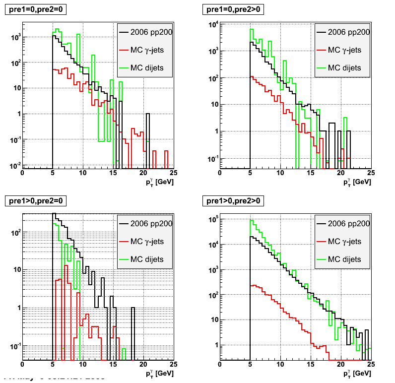
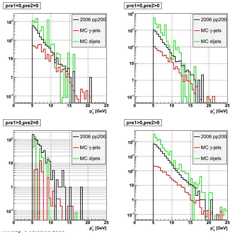
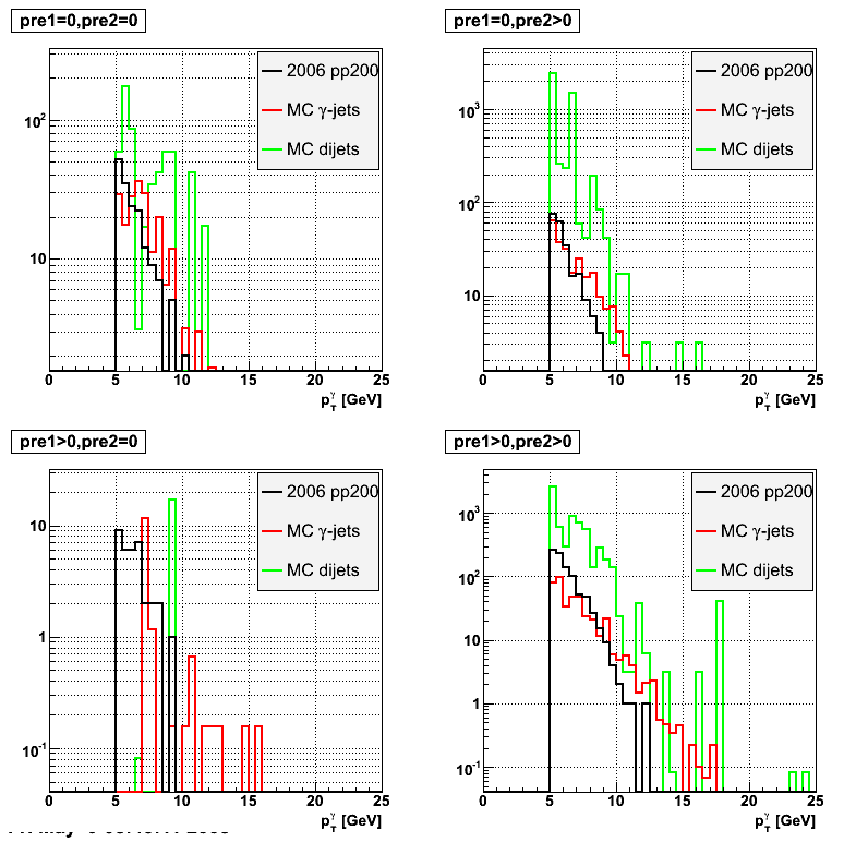
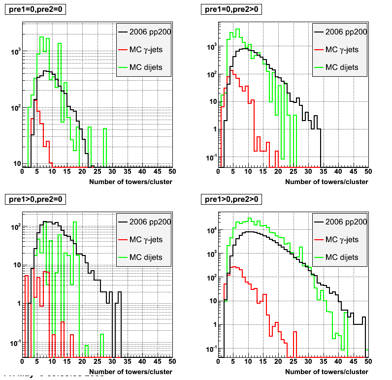
2008.04.12 Data-Driven Residuals

Data-Driven Residuals

Gammas

Jets

Background Rejection vs. Signal Efficiency

Partonic p_T=9-11 GeV	Partonic p_T=9-11 GeV

Background Rejection vs. Signal Efficiency (Neutral Meson pT > 8 GeV)

Pibero Djawotho

Last updated Sat Apr 12 13:27:50 EDT 2008

2008.04.12 Pythia Gamma-Jets

Pythia Gamma-Jets

Gamma-Jet Yields

During Run 6, the L2-gamma trigger (trigger id 137641) sampled 4717.10 nb^-1 of integrated luminosity. By restricting the jet to the Barrel, |η_jet|<1, and the gamma to the Endcap, 1<η_gamma<2, the yield of gamma-jets is estimated as the product of the luminosity, the cross section, and the fraction of events in the phasespace above. The total cross section reported by Pythia for gamma-jet processes at different partonic p_T thresholds is listed in the table below. No efficiencies are included.

p_T threshold [GeV]	Total cross section [mb]	Fraction	N_gamma-jets
5	6.551E-05	0.0992	30654
6	3.075E-05	0.1161	16840
7	1.567E-05	0.1150	8500
8	8.654E-06	0.1131	4617
9	4.971E-06	0.1223	2868
10	2.953E-06	0.1151	1603

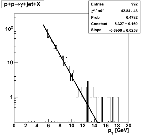
Gamma-Jets p_T slope

The p_T slope is exp(-0.69*pT)=2^(-pT), so the statistics are halved with each 1 GeV increase in p_T.

References

Pibero Djawotho

Last updated Sat Apr 12 15:15:56 EDT 2008

2008.04.16 Jet Finder QA

Jet Finder QA

Pibero Djawotho

Last updated Wed Apr 16 08:33:01 EDT 2008

2008.04.20 BUR 2009

Partonic pT=7-9 GeV

Partonic pT=9-11 GeV

Combined Partonic pT

2008.04.22 Run 6 Photon Yield Per Trigger

Run 6 Photon Yield Per Trigger

Introduction

The purpose of this study is to estimate the photon yield per trigger in the Endcap Electromagnetic Calorimeter during Run 6. The trigger of interest is the L2-gamma trigger. Details of the STAR triggers during Run 6 were compiled in the 2006 p+p run (run 6) Trigger FAQ by Jamie Dunlop. The triggers relevant to this study are reproduced in the table below for convenience.

Trigger id	Trigger name	Description
117641	eemc-http-mb-l2gamma	EEMC HT > th1 (12, 2.6 GeV) and TP > TH1 (17, 3.8 GeV), minbias condition, L2 Gamma algorithm, reading out slow detectors, L2 thresholds at 2.9, 4.5
127641	eemc-http-mb-l2gamma	EEMC HT > th1 (12, 2.6 GeV, run < 7100052;13, 2.8 GeV, run >=7100052) and TP > TH1 (17, 3.8 GeV, run < 710052; 21, 4.7 GeV, run>=7100052 ), minbias condition, L2 Gamma algorithm, reading out slow detectors, L2 thresholds at 3.4, 5.4, transverse running
137641	eemc-http-mb-l2gamma	EEMC HT > th1 (16, 3.5 GeV) and TP > th1 (20, 4.5 GeV), minbias condition, L2 Gamma algorithm, reading out slow detectors, L2 thresholds at 3.7, 5.2, longitudinal running 2

The luminosity sampled by each trigger was also caclulated here by Jamie Dunlop. The luminosity for the relevant triggers is reproduced in the table below for convenience. The figure-of-merit (FOM) is calculated as FOM=Luminosity*P_B*P_Y for transverse runs and FOM=Luminosity*P_B²*P_Y² for longitudinal runs where P_B is the polarization of the blue beam and P_Y is the polarization of the yellow beam. Naturally, in spin physics, the FOM is the better indicator of statistical precisison.

Trigger	First run	Last run	Luminosity [nb^-1]	Figure-of-merit [nb^-1]
117641	7093102	7096017	118.88	11.89
127641	7097009	7129065	3219.04	1099.43
137641	7135050	7156028	4717.10	687.65

Event selection

Trigger selection

For this study, only the trigger of longitudinal running 2 (137641) is used. As mentioned above, at level-0, an EEMC high tower above 3.5 GeV and its associated trigger patch above 4.5 GeV in transverse energy coupled with a minimum bias condition, which is simply a BBC coincidence to ensure a valid collision, is required for the trigger to fire. The EEMC has trigger patches of variable sizes depending on their location in pseudorapidity. (The BEMC has trigger patches of fixed sizes, 4x4 towers.) At level-2, a high tower above 3.7 GeV and a 3x3 patch above 5.2 GeV in transverse energy is required to accept the event.

Gamma candidates

In addition to selecting events that were tagged online by the L2-gamma trigger, the offline

StGammaMaker

looks for tower clusters with minimum transverse energy of 5 GeV. These clusters along with their associated TPC tracks, preshower and postshower tiles, and SMD strips form gamma candidates. Gamma trees for the 2006 trigger ID 137641 with primary vertex are located at

/star/institutions/iucf/pibero/2006/gammaTrees/

.

Track isolation

The gamma candidate is required to have no track pointing to any of its towers.

EMC isolation

The gamma candidate is required to have 85% of the total transverse energy in a cone of radius 0.3 in eta-phi space around the position of the gamma candidate. That is E

_T^gamma

/E

_T^cone

> 0.85 and R=√Δη

²

+Δφ

²

=0.3 is the cone radius.

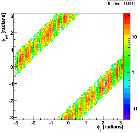
Jet Reconstruction

The gamma candidate is matched to the best away-side jet with neutral fraction < 0.9 and cos(φ

_gamma

-φ

_jet

) < -0.8. The 2006 jet trees are produced by Murad Sarsour at PDSF in

/eliza13/starprod/jetTrees/2006/trees/

. A local mirror exists at RCF under the directory

/star/institutions/iucf/pibero/2006/jetTrees/

.

Spin Information

Jan Balewski has an excellent write-up, Offline spin DB at STAR, on how to get spin states. I obtain the spin states from the skim trees in the jet trees directory. In brief, the useful spin states are:

Blue Beam Polarization	Yellow Beam Polarization	Spin4
P	P	5
P	N	6
N	P	9
N	N	10

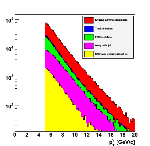
Event Summary

L2-gamma triggers	730128
Endcap gamma candidates	723848
Track isolation	246670
EMC isolation	225400
Away-side jet	99652
SMD max sided residual	19281
Barrel-only jet	15638

Note the number of L2-gamma triggers include only those events with a primary vertex and at least one gamma candidate (BEMC or EEMC).

Gamma-Jet Plots

Comparison of pT Slope with Pythia

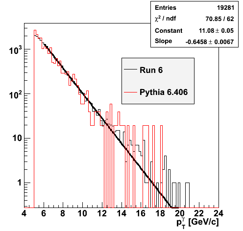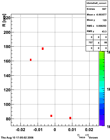
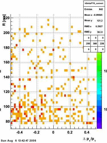
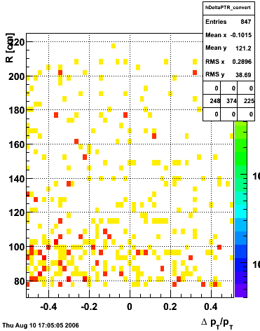
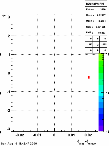
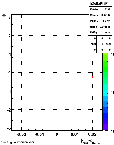
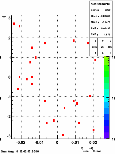
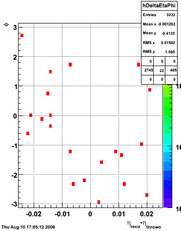
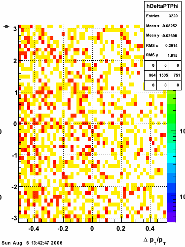
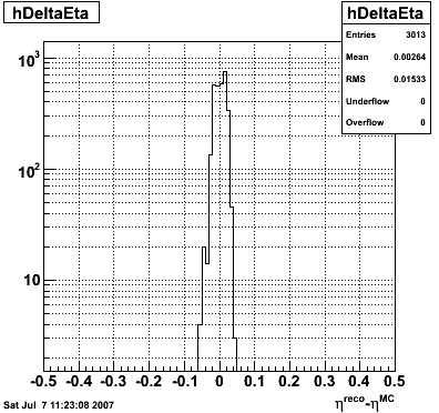
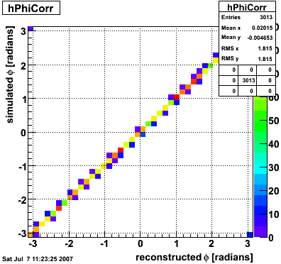
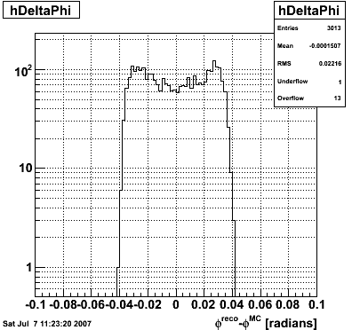
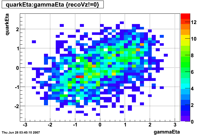
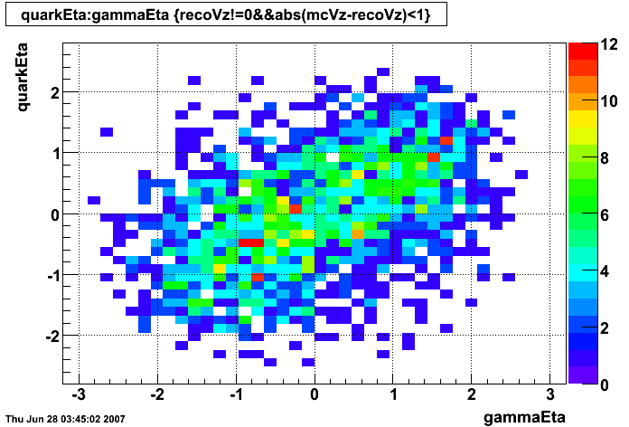
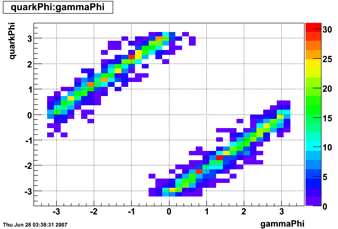
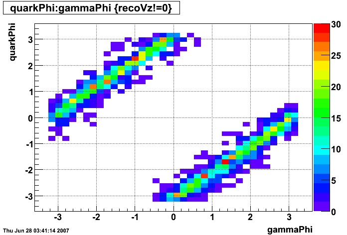
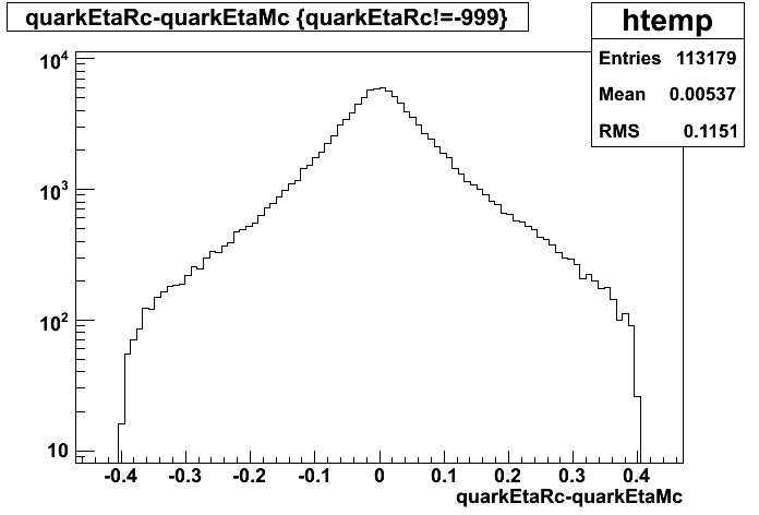
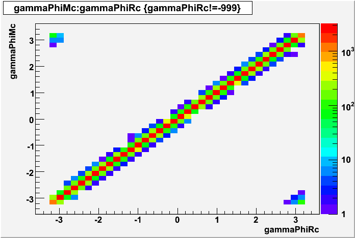
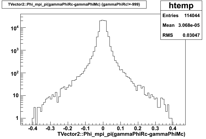
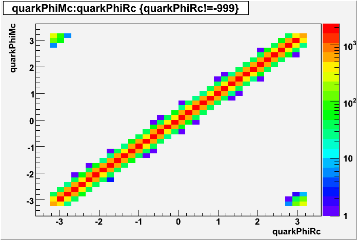
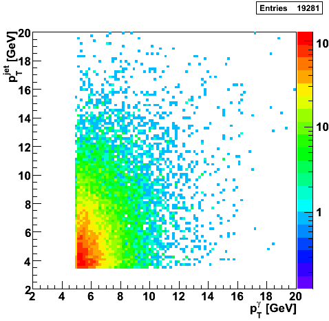
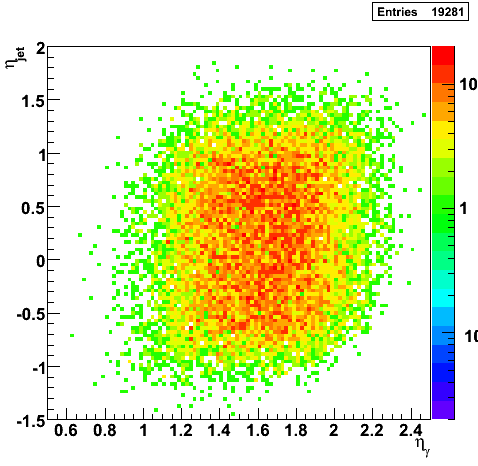
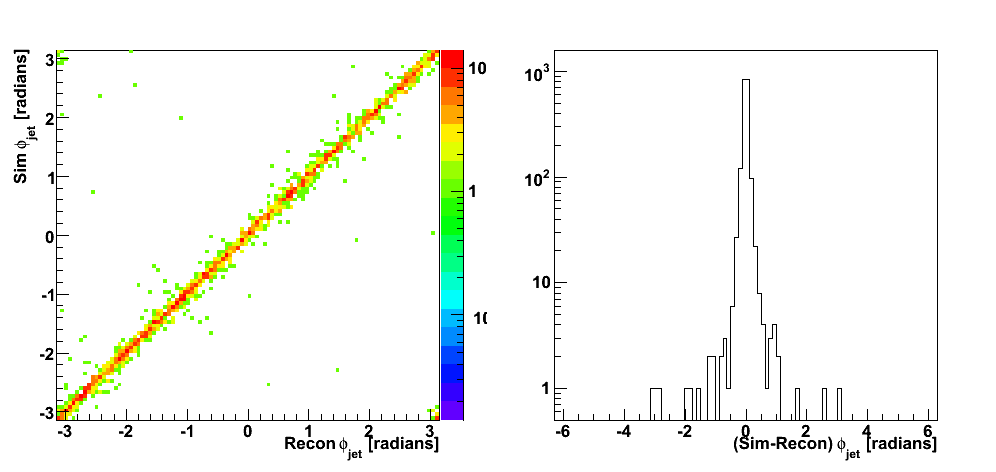
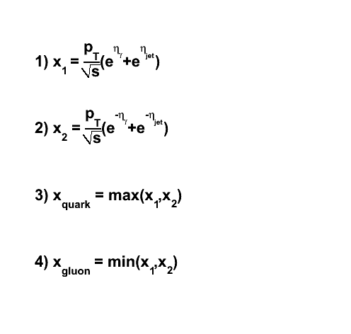
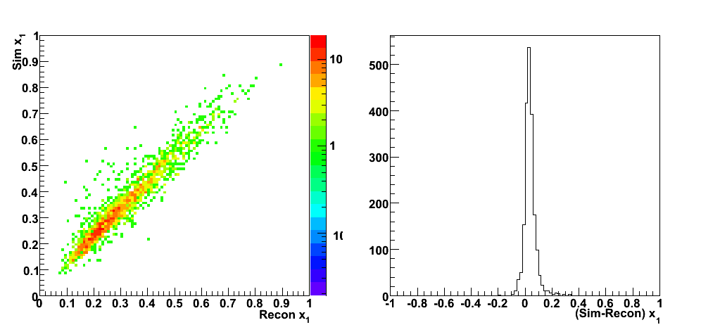
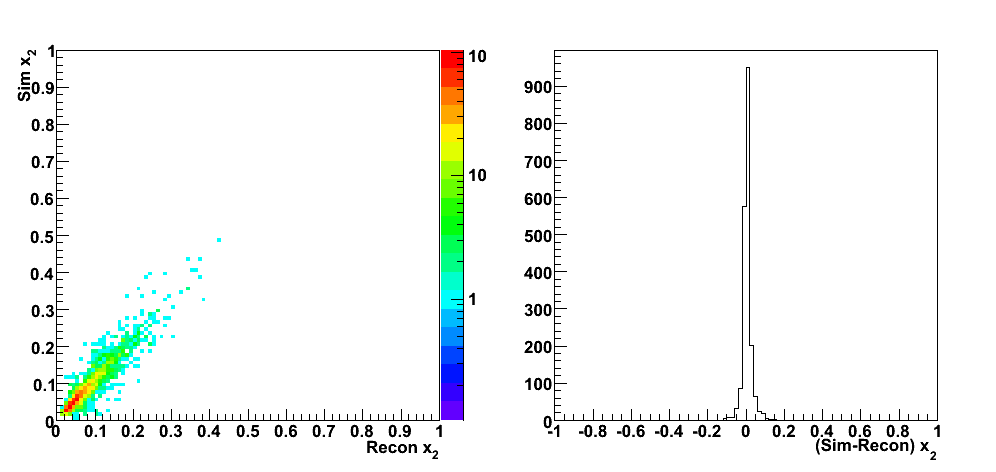
Partonic Kinematics Reconstruction

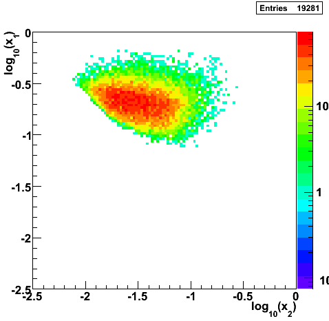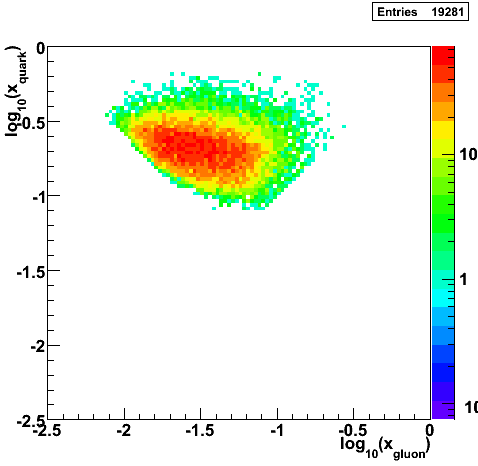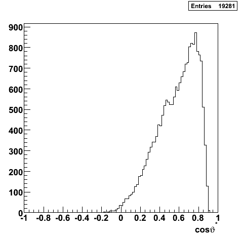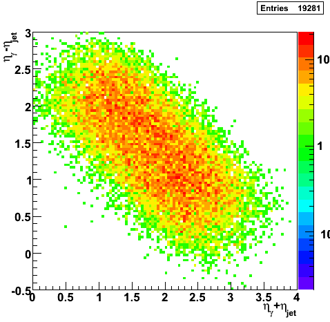Open Questions

I count ~2.4M events with trigger id 137641 using the Run 6 Browser, however my analysis only registers about ~0.78M.

Pibero Djawotho

Last updated Tue Apr 22 11:40:18 EDT 2008

2008.05.07 Number of Jets

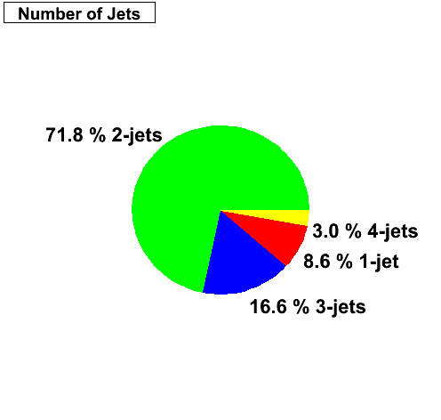
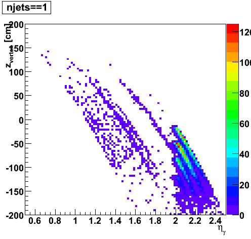
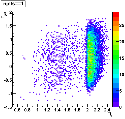
Number of Jets

After selecting Endcap gamma candidates out of L2-gamma triggers, applying track and EMC isolation cuts, and matching the Endcap gamma candidate to an away-side jet, I record the number of jets below per event. Surprisingly, 8% of the events only have 1 jet. Those are events where the Endcap gamma candidate was not reconstructed as a neutral jet by the jet finder. The question is why.

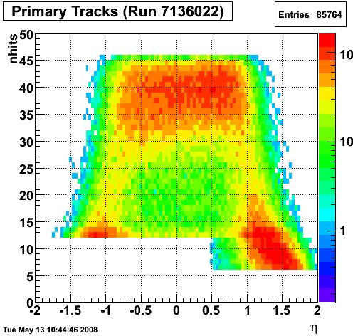I display both Barrel and Endcap calorimeter towers (the z-axis represents tower energy) and draw a circle of radius 0.3 around the gamma candidate and a circle of radius 0.7 around the away-side jet for 2006 pp200 run 7136022. Even though many of the gamma candidates not reconstructed by the jet finder are at the forward edge of the Endcap, it is not at all clear why those that are well within the detector are not being reconstructed.

Pibero Djawotho

Last updated Wed May 7 09:54:32 EDT 2008

2008.05.09 Gamma-jets pT distributions

Gamma-jets pT distributions

Note:

No cuts on residuals applied.

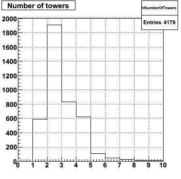
Not cut on number of towers in gamma cluster

Number of towers in gamma cluster <= 9

Number of towers in gamma cluster <= 4

Number of towers per cluster distributions

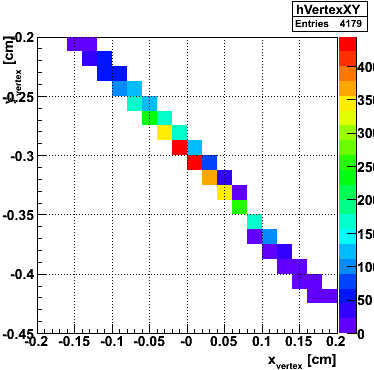
Gamma candidates xy-distribution

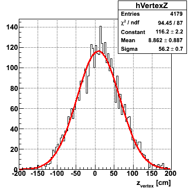
z-vertex distribution

Eta distribution

Phi distribution

log10(E_post/E_tow) distribution

pT asymmetry

References

Pibero Djawotho

Last updated Fri May 9 08:19:00 EDT 2008

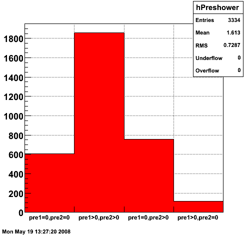
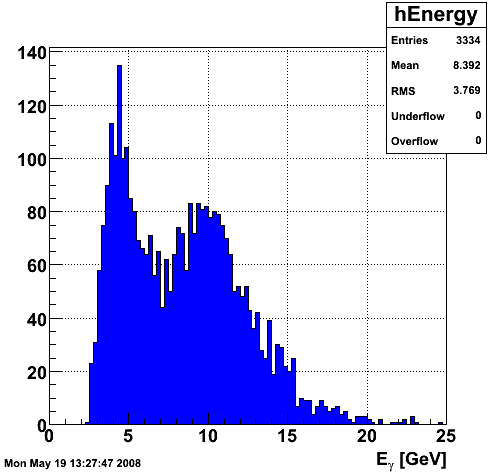
2008.05.19 Binning the shower shape library

Binning the shower shape library

Distributions

Shower Shapes

Pibero Djawotho

Last updated Mon May 19 12:09:48 EDT 2008

2008.06.03 Jet A_LL Systematics

Jet A_LL Systematics

Hypernews discussion

jet A_LL systematic possibility

References

Pibero Djawotho

Last updated Tue Jun 3 15:35:24 EDT 2008

2008.06.18 Photon-jet reconstruction with the EEMC - Part 2 (STAR Collaboration Meeting - UC Davis)

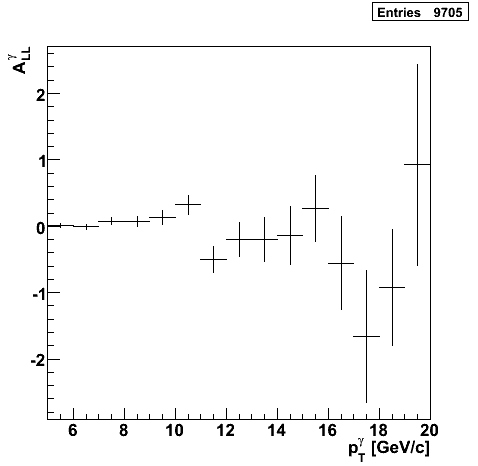
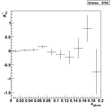
2008.07.16 Extracting A_LL and DeltaG

Extracting A_LL and DeltaG

Determining state of beam polarization for Monte Carlo events

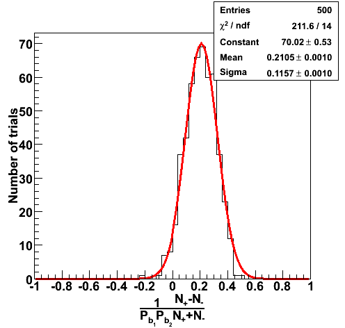
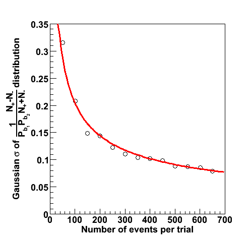
While Pythia does a pretty good job of simulating prompt photon production in p+p collisions, it does not include polarization for the colliding protons nor partons. A statistical method for assigning polarization states for each event based on A_LL [1] is demonstrated in this section. For an average number of interactions for each unpolarized bunch crossing, N_eff, the occurence of an event with a particular polarization state obeys a Poisson distribution with average yield of events per bunch crossing:

For simplicity, the polarizations of the blue and yellow beams are assumed to be P

_B

=P

_Y

=0.7 and N

_eff

=0.01. The "+" spin state defines the case where both beams have the same helicities and the "-" spin state for the case of opposite helicities. The asymmetry A

_LL

is calculated from the initial states polarized and unpolarized parton distribution functions and parton-level asymmetry:

The algorithm then consists in alternatively drawing a random value N

_int

from the Poisson distributions with mean μ

₊

and μ

_-

until N

_int

>0 at which point an interaction has occured and the event is assigned the current spin state. The functioning of the algorithm is illustrated in Figure 1a where an input A

_LL

=0.2 was fixed and N

_trials

=500 different asymmetries were calculated. Each trial integrated N

_total

=300 events. It is then expected that the mean A

_LL

~0.2 and the statistical precision~0.1:

Indeed, both the A

_LL

and its error are reproduced. In addition, variations on the number of events per trial were investigated (N

_total

) in Figure 1b. The extracted width of the Gaussian distribution for A

_LL

is consistent with the prediction for the error (red curve).

ROOT macro used to generate Figure 1a SimALL.C
ROOT macro used to generate Figure 1b SimALL2.C

Figure 1a	Figure 1b

Event reconstruction

For this study, the gamma-jets Monte Carlo sample for all partonic p_T were used. As an example, the prompt photon processes for the partonic p_T bin 9-11 GeV and their total cross sections are listed in the table below. Each partonic p_T bin was divided into 15 files each of 2000 events.

 ==============================================================================
 I                                  I                            I            I
 I            Subprocess            I      Number of points      I    Sigma   I
 I                                  I                            I            I
 I----------------------------------I----------------------------I    (mb)    I
 I                                  I                            I            I
 I N:o Type                         I    Generated         Tried I            I
 I                                  I                            I            I
 ==============================================================================
 I                                  I                            I            I
 I   0 All included subprocesses    I         2000          9365 I  3.074E-06 I
 I  14 f + fbar -> g + gamma        I          331          1337 I  4.930E-07 I
 I  18 f + fbar -> gamma + gamma    I            2             8 I  1.941E-09 I
 I  29 f + g -> f + gamma           I         1667          8019 I  2.579E-06 I
 I 114 g + g -> gamma + gamma       I            0             1 I  1.191E-10 I
 I 115 g + g -> g + gamma           I            0             0 I  0.000E+00 I
 I                                  I                            I            I
 ==============================================================================

The cross sections for the different partonic p_T bins has been tabulated by Michael Betancourt and is reproduced here for convenience.

Partonic p_T [GeV]	Cross Section [mb]
3-4	0.0002962
4-5	0.0000891
5-7	0.0000494
7-9	0.0000110
9-11	0.00000314
11-15	0.00000149
15-25	0.000000317
25-35	0.00000000990
35-45	0.000000000449

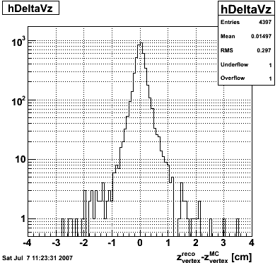
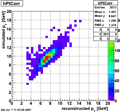
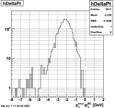
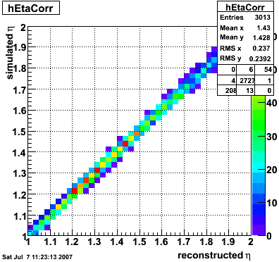
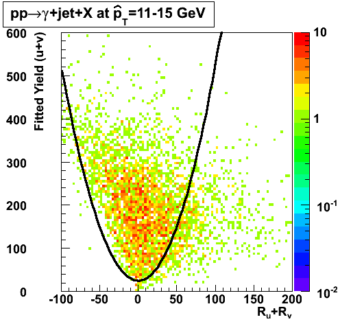
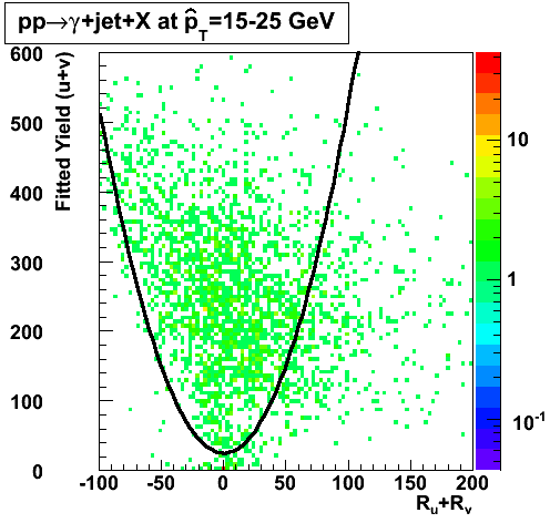
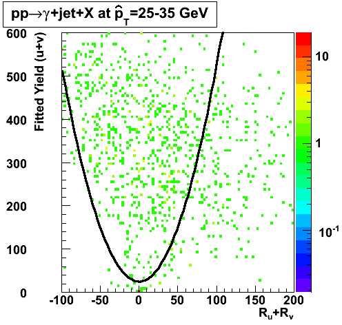
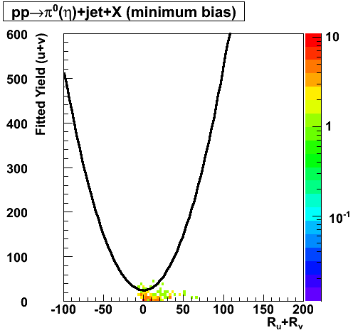
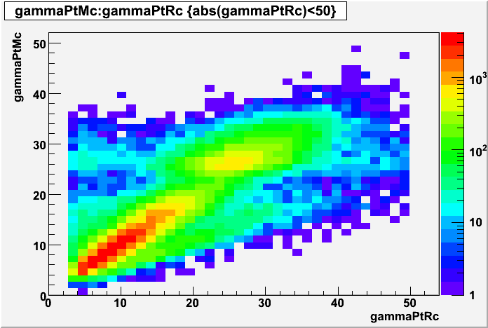
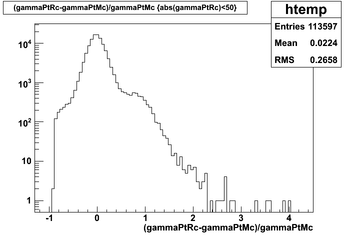
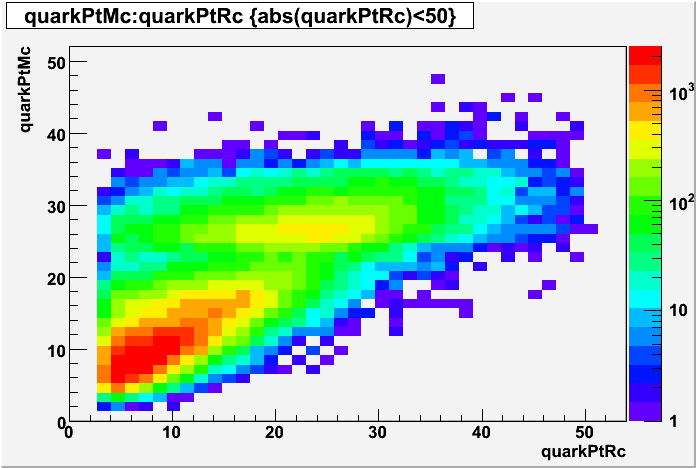
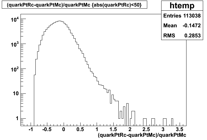
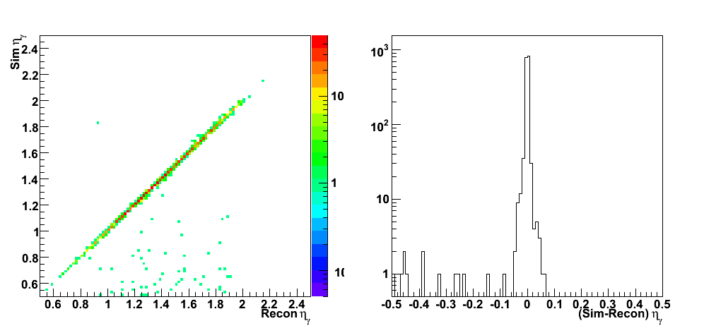
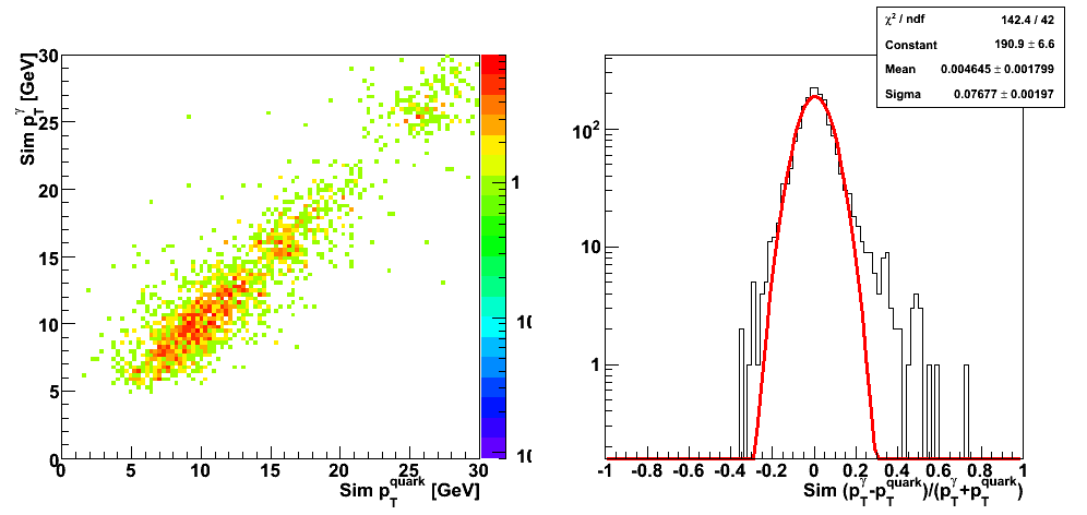
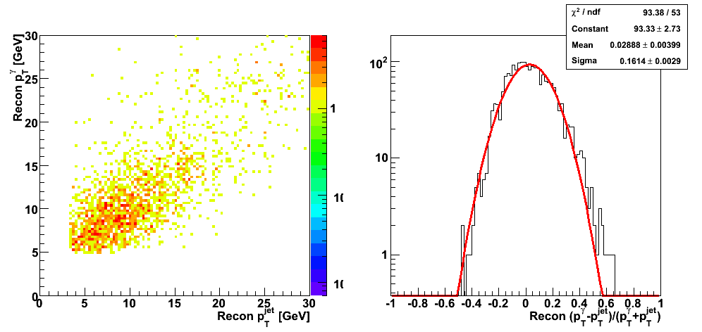
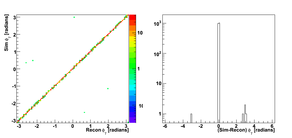
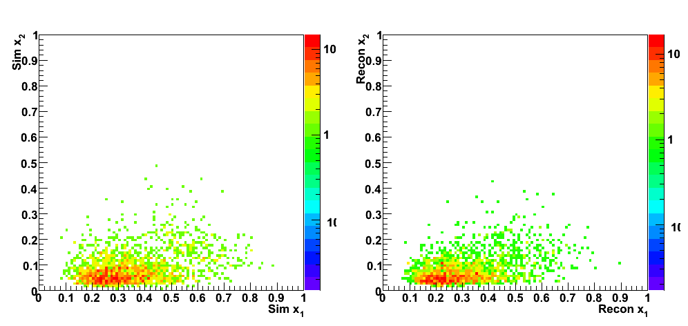
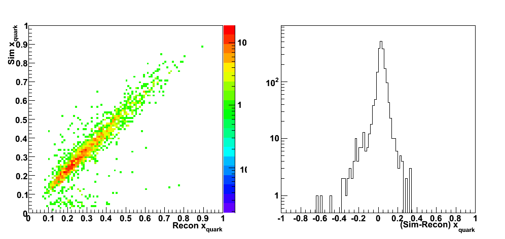
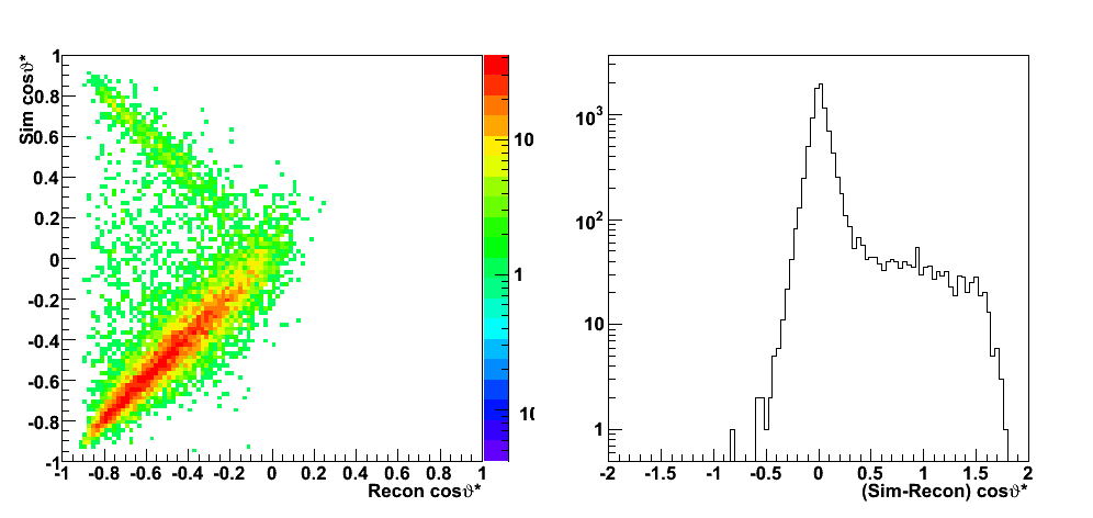
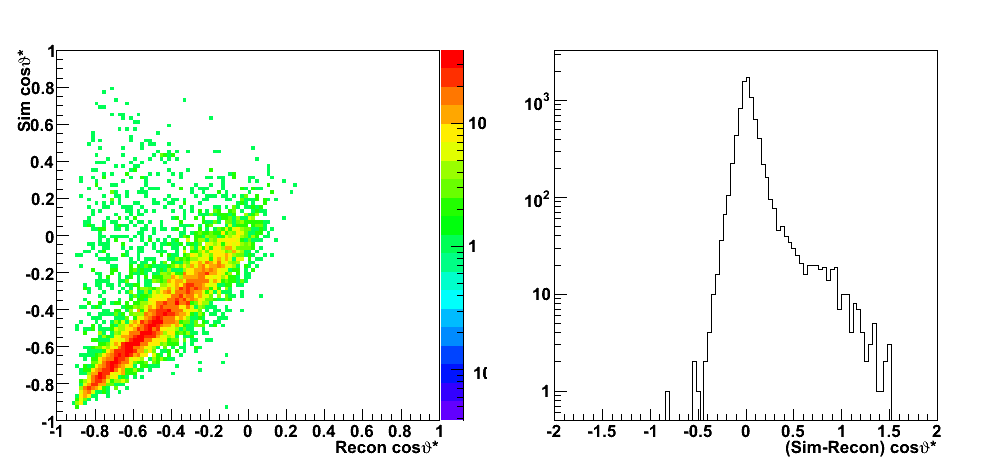
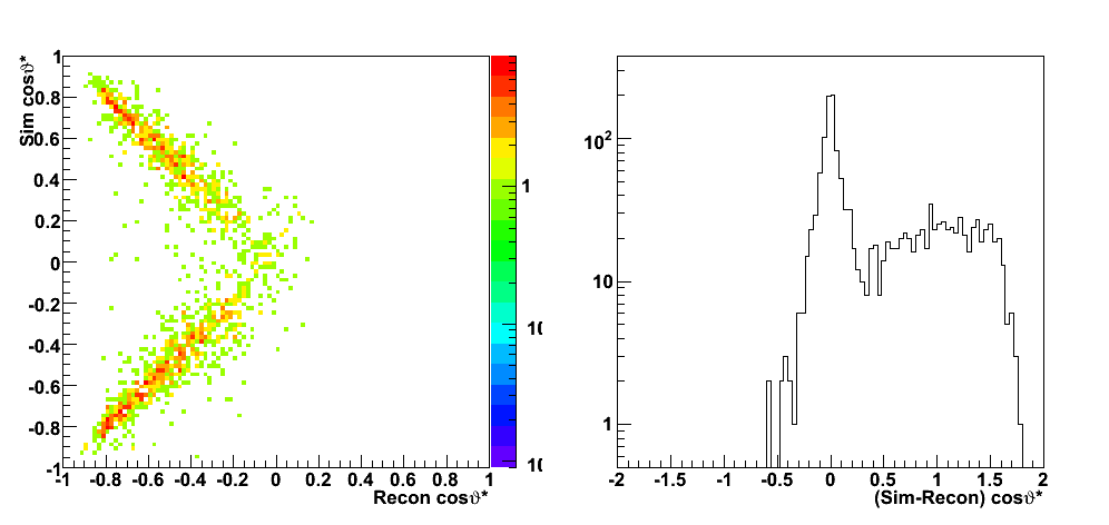
These events were processed through the 2006 pp200 analysis chain, albeit without any cuts on the SMD. The simulated quantities were taken from the Pythia record and the reconstructed ones from the analysis.

Figure 2

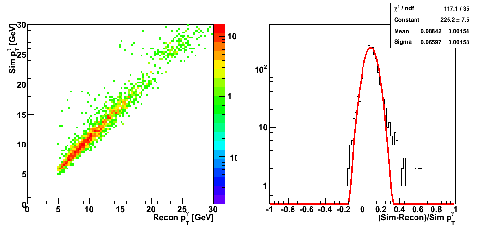Figure 3

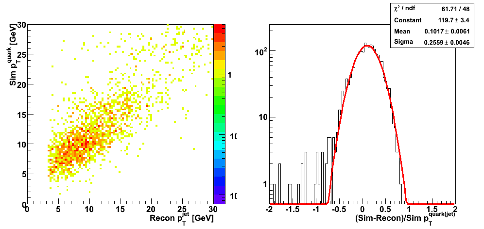Figure 4

Figure 5

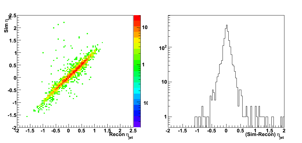Figure 6

Figure 7

Figure 8

Figure 9

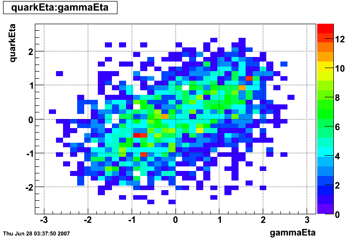
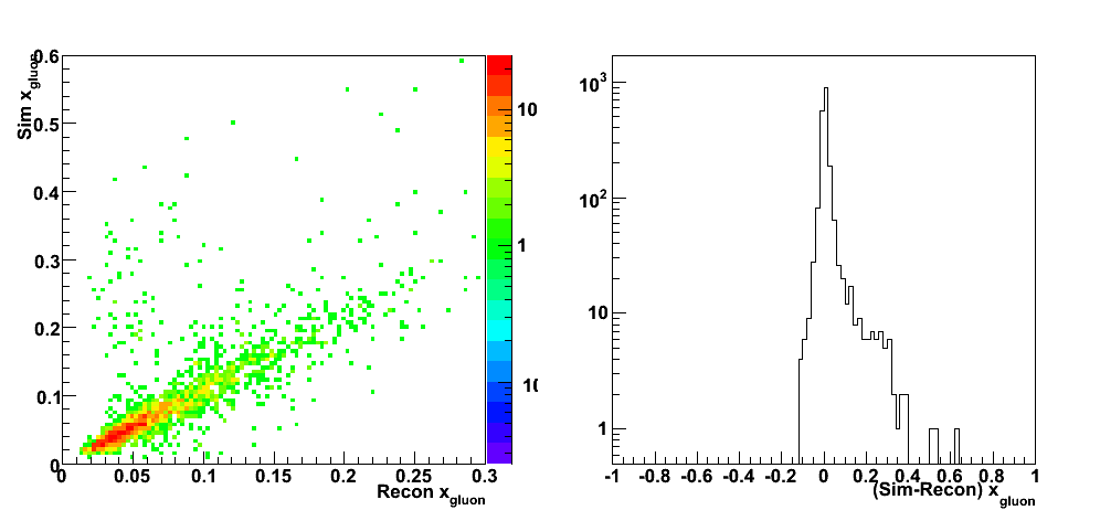
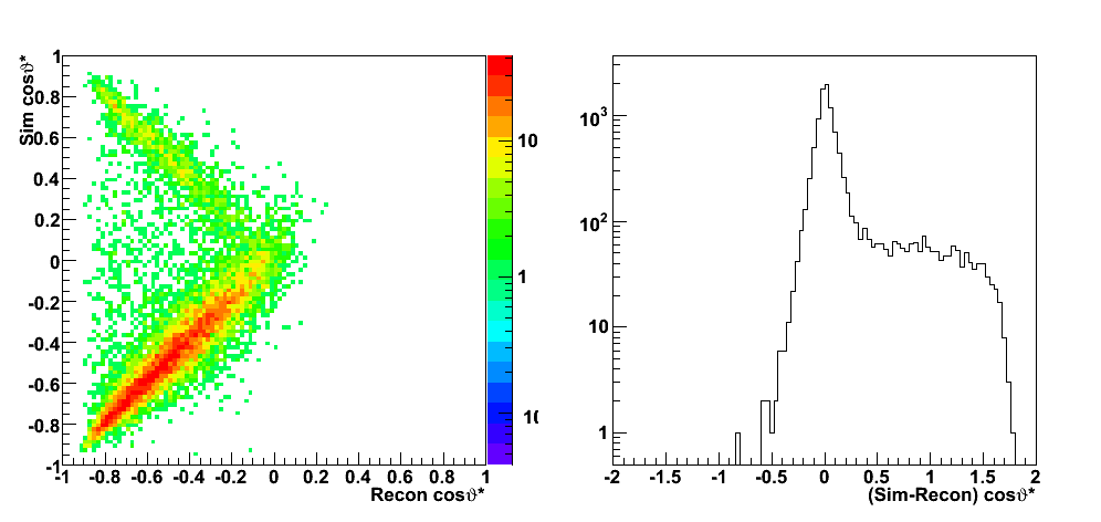
Partonic kinematics reconstruction

PartonicKinematics.C

Figure 10

Figure 11

Figure 12

Figure 13

Figure 14

Figure 15 (a)

Figure 15 (b): quark from proton 1 (blue beam, +z direction)

Figure 15 (c): quark from proton 1 (blue beam, +z direction) and q + g -> q + gamma subprocess (29)

Figure 15 (d): quark from proton 1 (blue beam, +z direction) and q + qbar -> gamma + g subprocess (14)

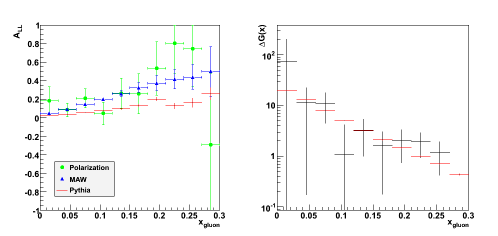
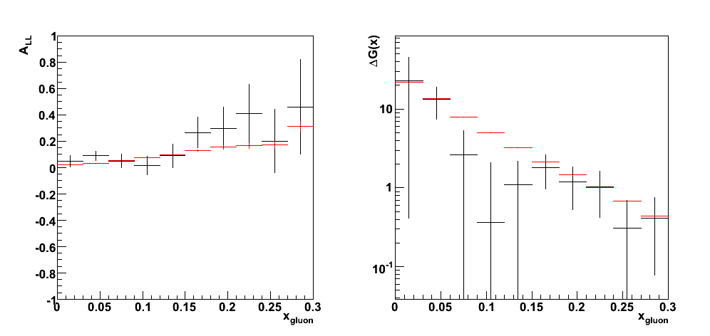
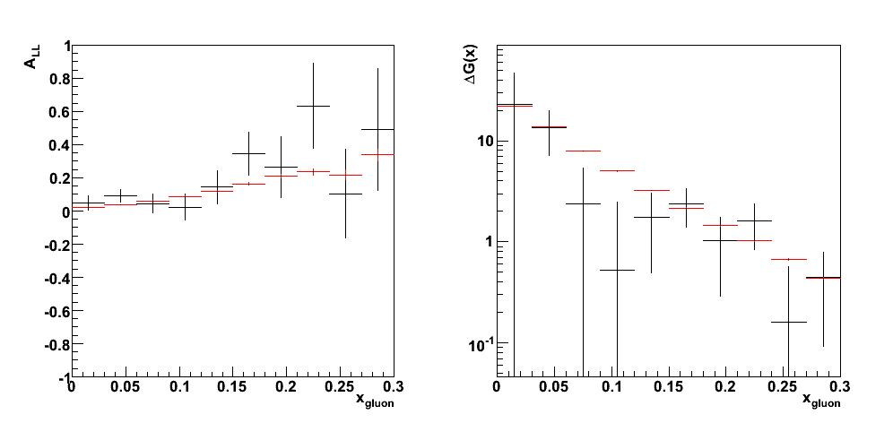
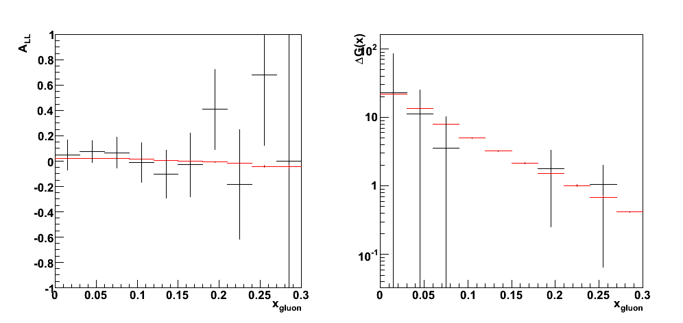
Predictions for A_LL and direct determination of DeltaG(x)

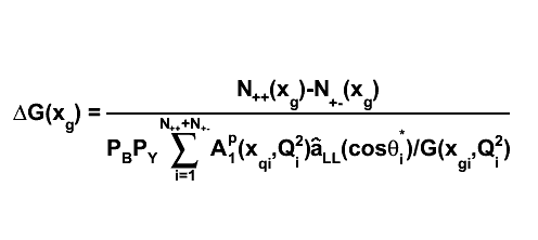DeltaG.C

Figure 16 (a)

Figure 16 (b): quark from proton 1 (blue beam, +z direction)

Figure 16 (c): quark from proton 1 (blue beam, +z direction) and q + g -> q + gamma subprocess (29)

Figure 16 (d): quark from proton 1 (blue beam, +z direction) and q + qbar -> gamma + g subprocess (14)

References

Pibero Djawotho

Last updated Wed Jul 16 10:29:22 EDT 2008

2008.07.20 How to install Pythia 6 and 8 on your laptop?

How to install Pythia 6 and 8 on your laptop?

Install Pythia 6 and build the interface to ROOT

pythia6.tar.gz

ftp://root.cern.ch/root/pythia6.tar.gz

tar zxvf pythia6.tar.gz

pythia6/

cd pythia6/
./makePythia6.linux

Installing ROOT from Source

Pythia Event Generators

Install Pythia 8

http://home.thep.lu.se/~torbjorn/Pythia.html

tar zxvf pythia8108.tgz

pythia8108/

README

PYTHIA8

PYTHIA8DATA

/etc/profile.d/pythia8.sh

export PYTHIA8=$HOME/pythia8108
export PYTHIA8DATA=$PYTHIA8/xmldoc

./configure --enable-shared
make

Install ROOT from source

http://root.cern.ch/

tar zxvf root_v5.20.00.source.tar.gz
cd root/
./configure linux --with-pythia6-libdir=$HOME/pythia6 \
  --enable-pythia8 \
  --with-pythia8-incdir=$PYTHIA8/include \
  --with-pythia8-libdir=$PYTHIA8/lib
make
make install

/etc/profile.d/root.sh

export ROOTSYS=/usr/local/root
export PATH=$PATH:$ROOTSYS/bin
export LD_LIBRARY_PATH=$LD_LIBRARY_PATH:$ROOTSYS/lib:/usr/local/pythia6
export MANPATH=$MANPATH:$ROOTSYS/man

root $ROOTSYS/tutorial/pythia/pythiaExample.C
root $ROOTSYS/tutorial/pythia/pythia8.C

Pibero Djawotho

Last updated on Sun Jul 20 23:35:39 EDT 2008

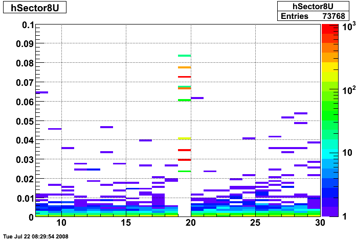
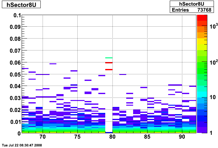
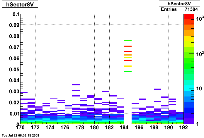
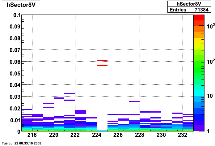
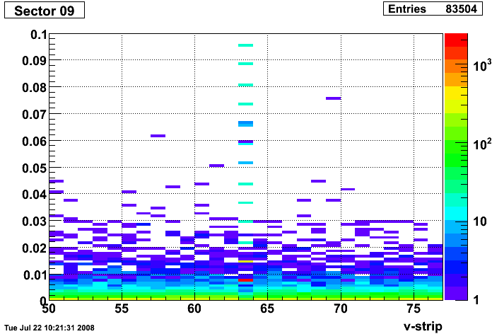
2008.07.23 Hot Strips Identified by Hal Spinka

Hot Strips Identified by Hal Spinka

Run 7136034 Sector 8

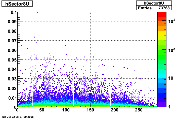
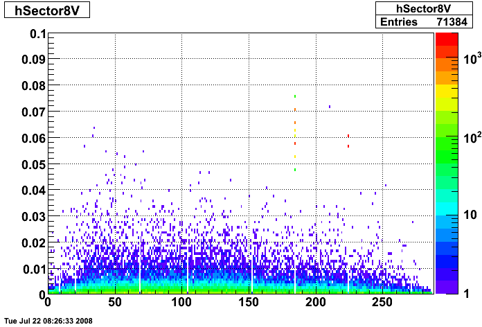
Strips 08U020, 08U080, 08V185 and 08V225

Run 7137036 Sector 9

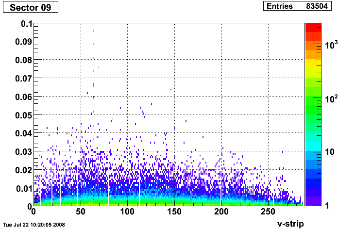
Strips 09V064

Pibero Djawotho

Last updated Wed Jul 23 03:40:54 EDT 2008

2008.07.24 Strips from Weihong's 2006 ppLong 20 runs

Strips from Weihong's 2006 ppLong 20 runs

Energy [GeV] vs. strip id

2006ppLongRuns.pdf

Raw ADC vs. strip id

7136022.pdf 7136033.pdf 7136034.pdf 7137036.pdf 7138001.pdf 7138010.pdf 7138032.pdf 7140046.pdf 7143012.pdf 7144014.pdf 7145018.pdf 7145024.pdf 7146020.pdf 7146077.pdf 7147052.pdf 7148027.pdf 7149005.pdf 7152062.pdf 7153008.pdf 7155052.pdf

Pibero Djawotho

Last updated Thu Jul 24 10:35:50 EDT 2008

EEMC Direct Photon Studies (Pibero Djawotho, 2006-2008)

2006.07.31 First Look at SMD gamma/pi0 Discrimination

Simulation

Maximal side residual

xy distribution of SMD hits

Single peak characteristics

Fit function

Single event SMD response

Code

Documents

2006.08.04 Second Look at SMD gamma/pi0 Discrimination

Second Look at SMD gamma/pi0 Discrimination

Dataset

Results

SMD U and V Fits

Code

2006.08.06 Comparison between EEMC fast and slow simulator

Comparison between EEMC fast and slow simulator

EEMC Fast Simulator

EEMC Slow Simulator

2006.09.15 Fit Parameters

Fit Parameters

Fit Function

Simulation

Fit Widths

Data from 2005 pp200 EEMC HT 1 and 2 triggers

Data from 2005 pp200 electrons

2007.02.05 Reconstructed/Monte Carlo Photon Energy

Reconstructed/Monte Carlo Photon Energy

Fit to a constant

Fit to a line

Fit to a quadratic

Comparison between Weihong's and Pibero's results

Constant

Linear

Quadratic

Conclusion

References

2007.02.08 E_reco / E_mc vs. eta

E_reco / E_mc vs. eta

Legend

Jason's Monte Carlo

Will's Monte Carlo

2007.02.11 Reconstructed/Monte Carlo Muon Energy

Reconstructed/Monte Carlo Muon Energy

zvertex

pT vs. η

EMC

Etower/EMC vs. η

Ecluster/EMC vs. η

Etowertanh(eta) vs. eta

2007.02.15 160 GeV photons

160 GeV photons

2007.02.15 20 GeV photons

20 GeV photons

2007.02.15 80 GeV photons

80 GeV photons

2007.02.15 Reconstructed/Monte Carlo Electron Energy

Reconstructed/Monte Carlo Electron Energy

E=1 GeV

E=2 GeV

2007.02.19 10 GeV photons

10 GeV photons

2007.02.19 40 GeV photons

40 GeV photons

2007.02.19 5 GeV photons

5 GeV photons

2007.02.19 Summary of Reconstructed/Monte Carlo Photon Energy

Summary of Reconstructed/Monte Carlo Photon Energy

Description

EEMC Fast/Slow Simulator Results

Conclusions

2007.05.24 gamma/pi0 separation in EEMC using linear cut

gamma/pi0 separation in EEMC using linear cut

2007.05.24 gamma/pi0 separation in EEMC using quadratic cut

gamma/pi0 separation in EEMC using quadratic cut

2007.05.24 gamma/pi0 separation in EEMC using quadratic cut

gamma/pi0 separation in EEMC using quadratic cut

2007.05.30 Efficiency of reconstructing photons in EEMC

Efficiency of reconstructing photons in EEMC

z_vertex

p_T vs. η

E_MC

E_tower/E_MC vs. η

E_cluster/E_MC vs. η

E_towertanh(eta) vs. eta

Partonic a_LL