QA Status (OBSOLETE)
The full list of STAR embedding requests (Since August, 2010):http://drupal.star.bnl.gov/STAR/starsimrequest
The QA status of each request can be viewed in its history.
The information below are only valid for OLD embedding requests.
This document is intended to provide all the information available for each production, starting for the last or current production.
P06ib
K star
Files: pdsf>/eliza1/starprod/embedding/KstarM* ( July 31 2007)Plots for Dedx, Mips, eta, phi distributions and vertex position on K star embedding are attached. Just around 20% of K star Minus files could be scanned due to space issues (in my home dir) at pdsf. Reconstructed tracks were done just on Daugther Pions. There is little difference(0.036) in the mips position possible due to lack of statistics.
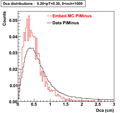
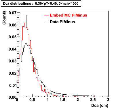
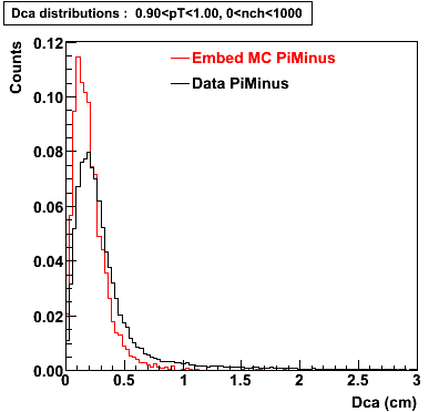
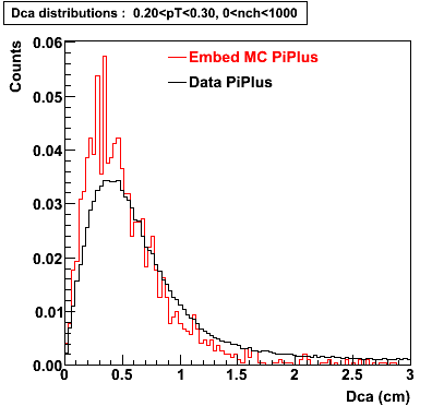
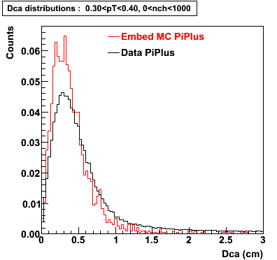
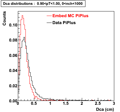
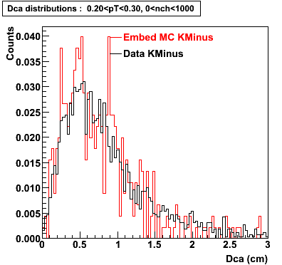
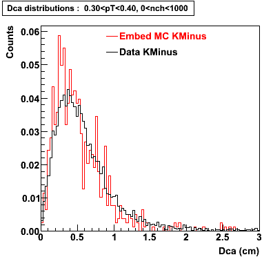
Plots - Dca Distributions
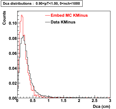
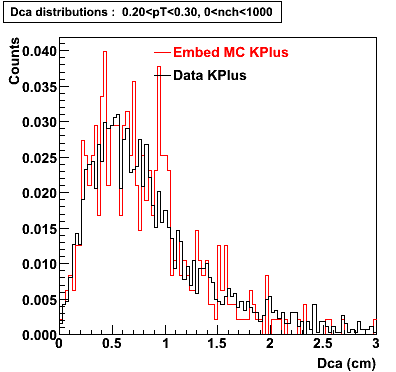
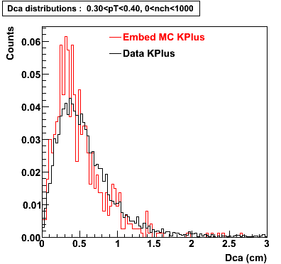
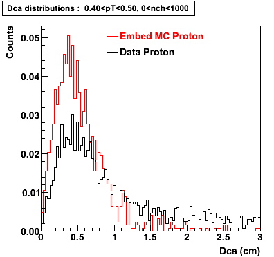
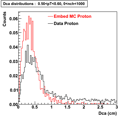
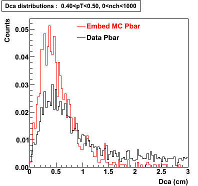
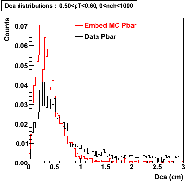
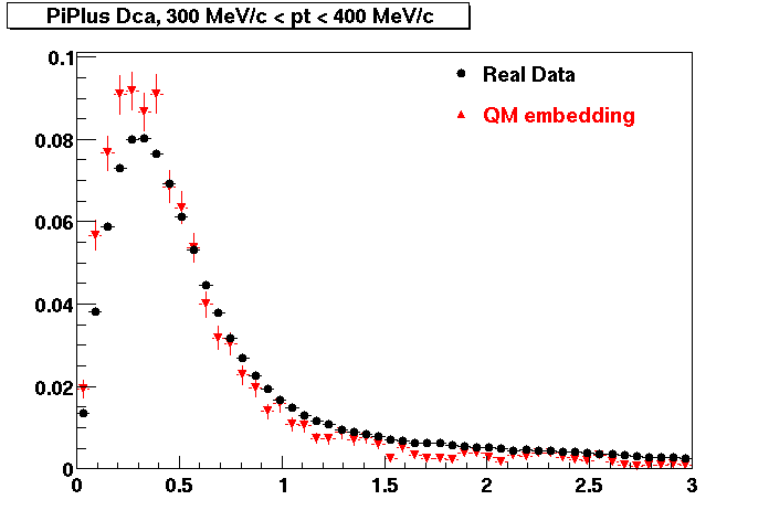
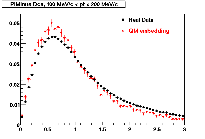
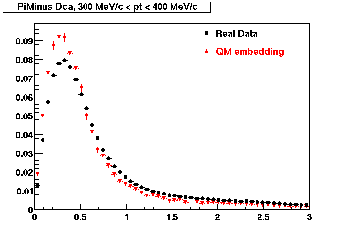
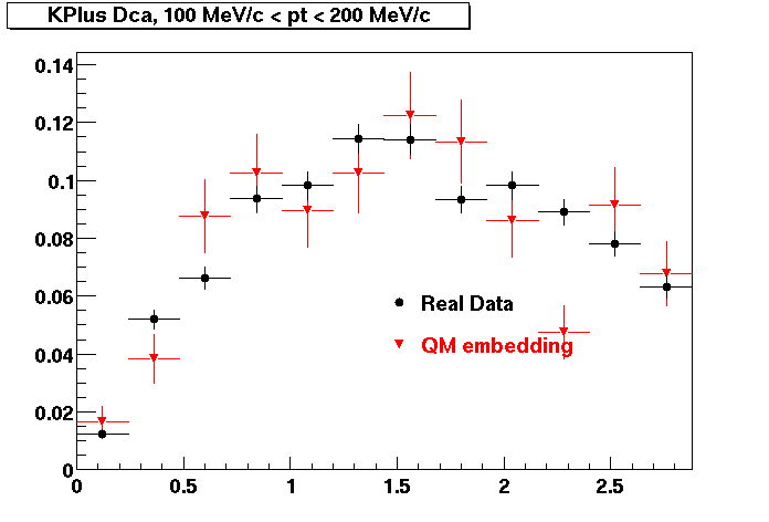
The Following are the results for dca distributions for different pT bins in Pi Minus. The results of dca agrees reasonable for the cut-off of 2 cm and above. These plots were done using the macro plot_dca.C
Event Selection Criteria
* Production: P06ib
* Vertex restriction: |x|<3.5cm, |y|<3.5cm, |z|<25.0cm
* N Fit points >= 25
* DCA < 3 cm
- PiMinus
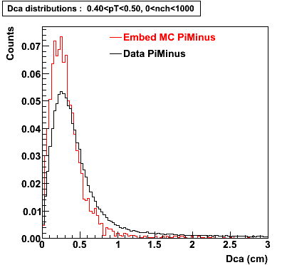

0.20<pT<0.30 0.30<pT<0.40 0.40<pT<0.50 0.50<pT<0.60 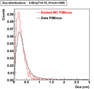
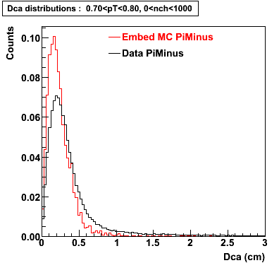
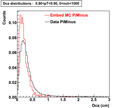
0.60<pT<0.70 0.70<pT<0.80 0.80<pT<0.90 0.90<pT<1.0
PiPlus
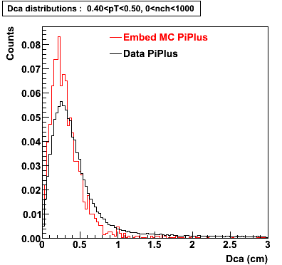
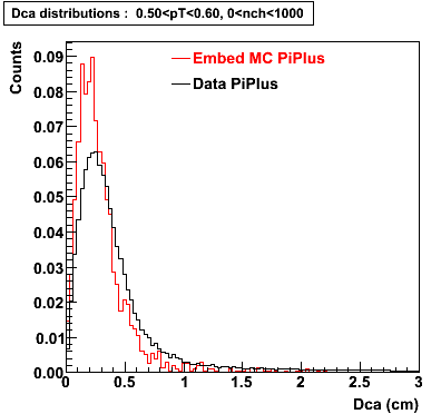
0.20<pT<0.30 0.30<pT<0.40 0.40<pT<0.50 0.50<pT<0.60 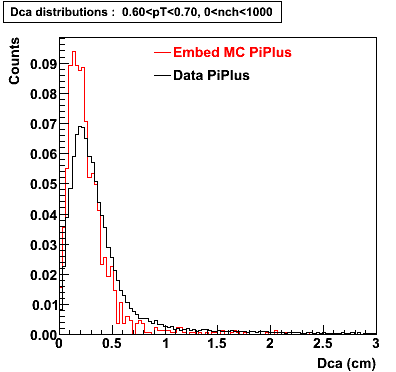
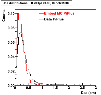
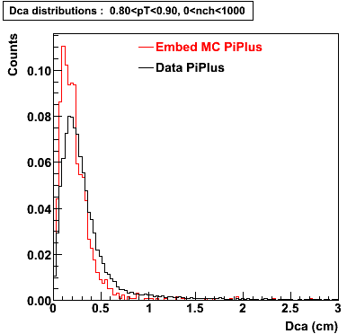
0.60<pT<0.70 0.70<pT<0.80 0.80<pT<0.90 0.90<pT<1.0
K Minus
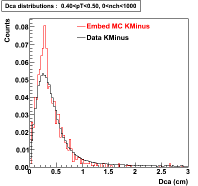
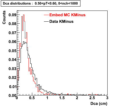
0.20<pT<0.30 0.30<pT<0.40 0.40<pT<0.50 0.50<pT<0.60 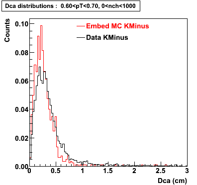

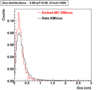
0.60<pT<0.70 0.70<pT<0.80 0.80<pT<0.90 0.90<pT<1.0
K Plus
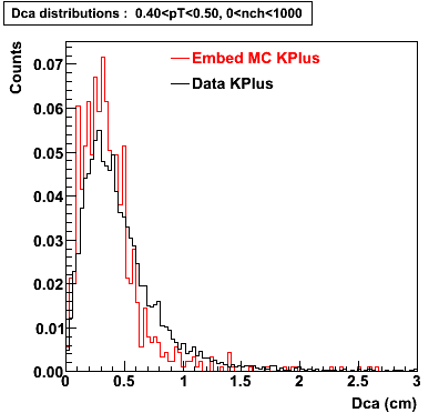
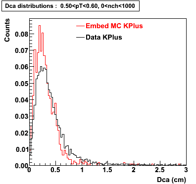
0.20<pT<0.30 0.30<pT<0.40 0.40<pT<0.50 0.50<pT<0.60 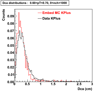

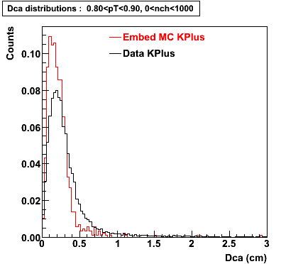
0.60<pT<0.70 0.70<pT<0.80 0.80<pT<0.90 0.90<pT<1.0
Proton
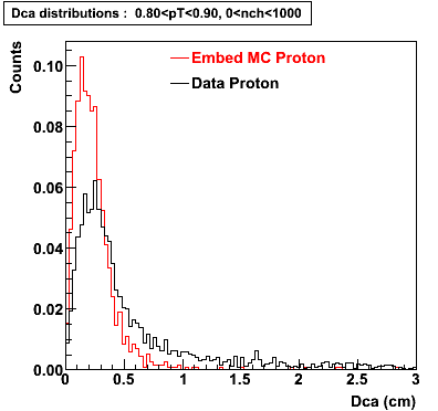
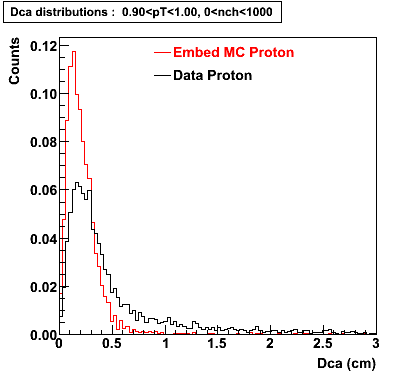
0.40<pT<0.50 0.50<pT<0.60 0.80<pT<0.90 0.90<pT<1.00
P bar
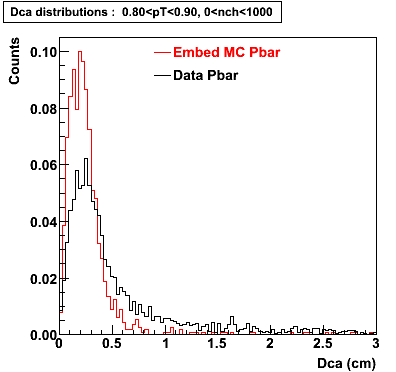
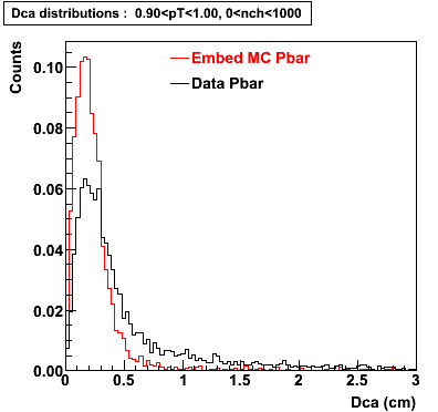
0.40<pT<0.50 0.50<pT<0.60 0.80<pT<0.90 0.90 < pT < 1.00
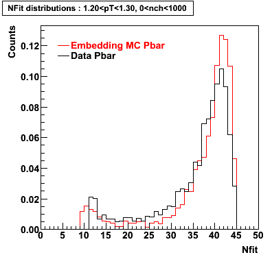
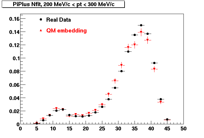
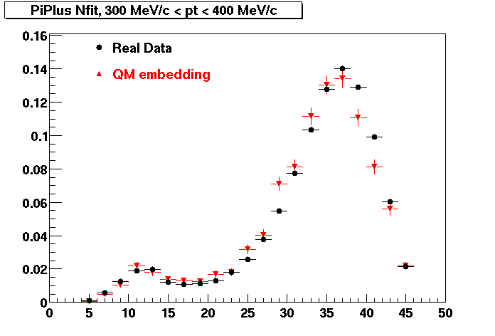
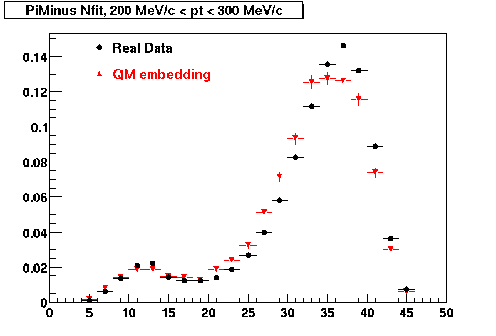
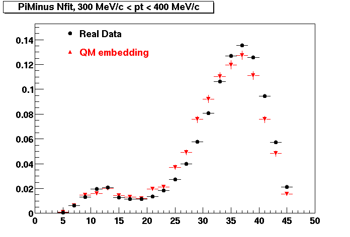
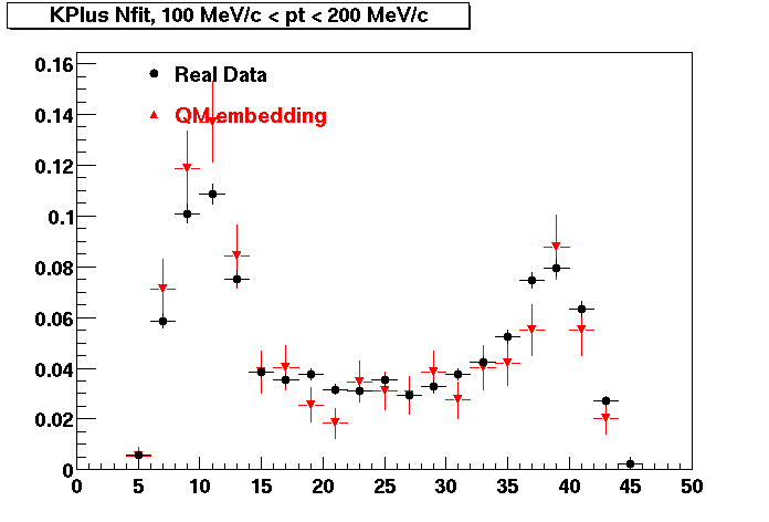
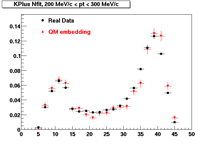
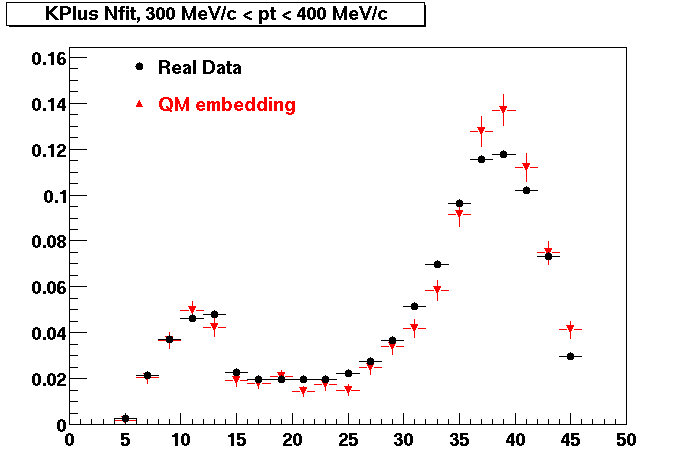
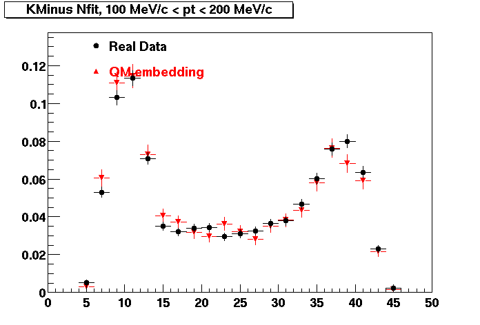
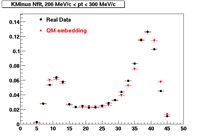
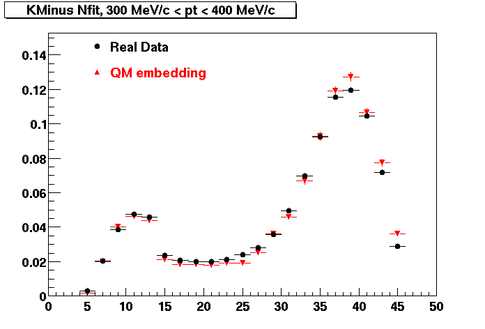
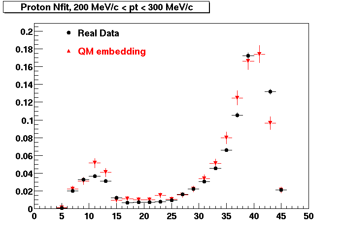
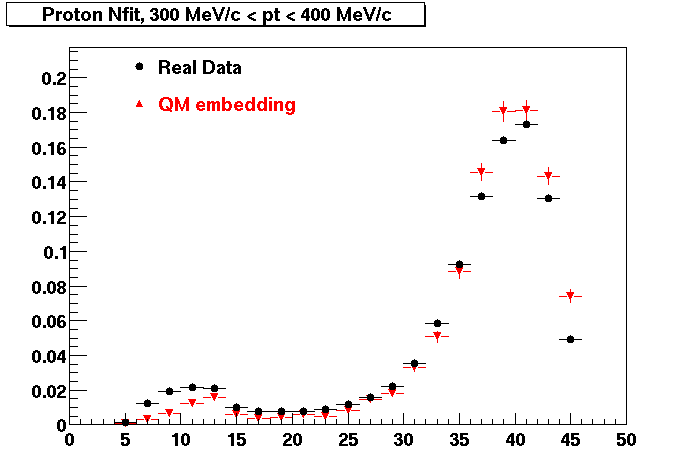
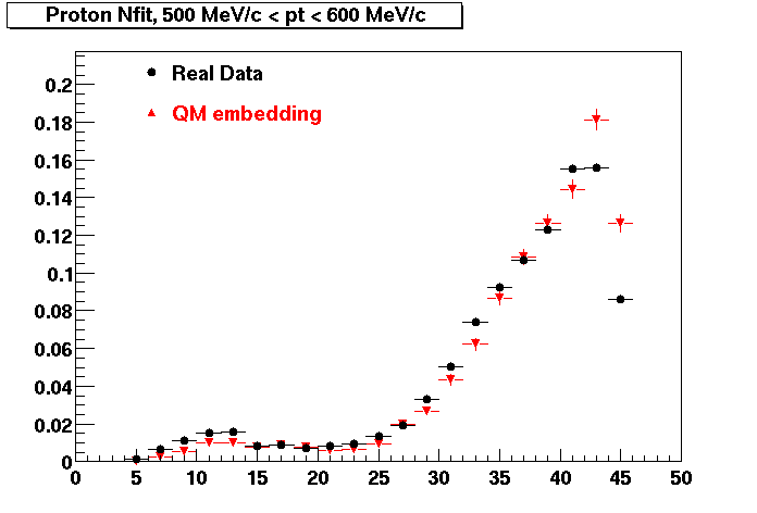
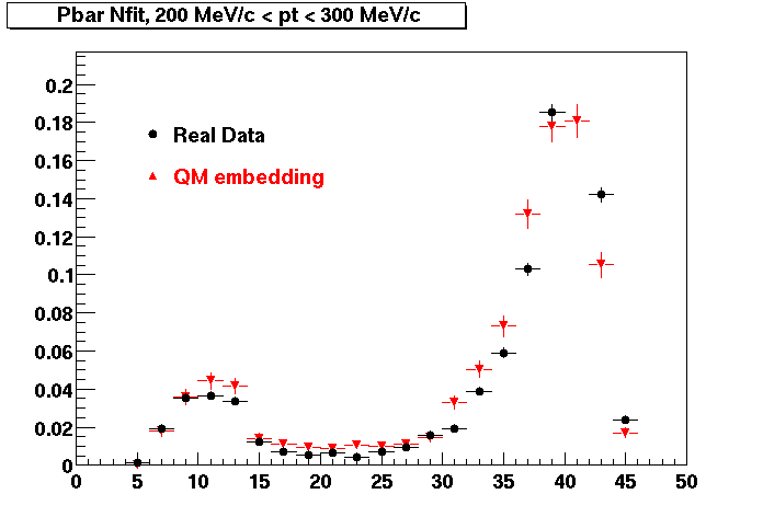
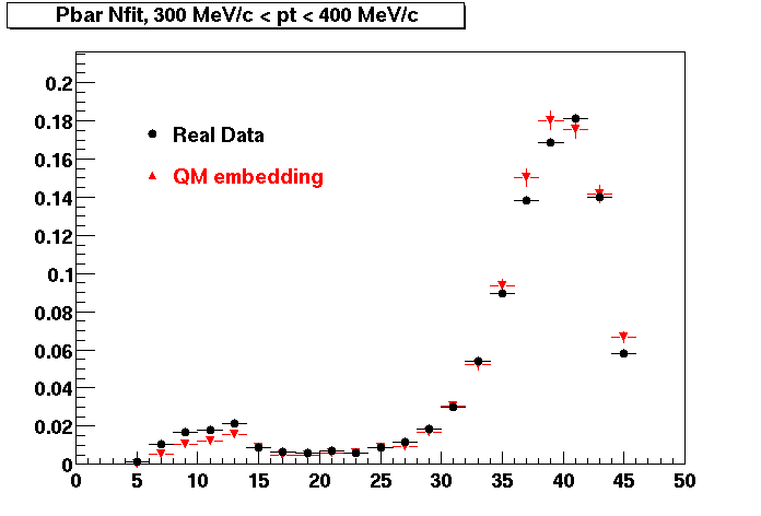
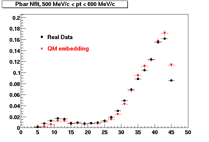
Plots - Number of Fitted Points
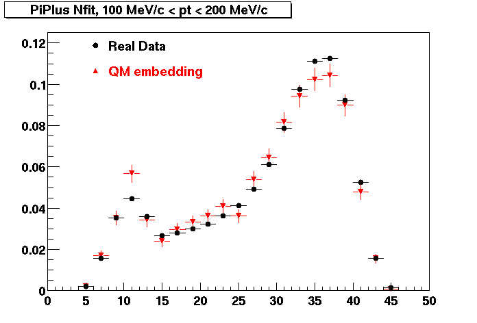
The Following are the results for dca distributions for different pT bins in Pi Minus. The results of dca agrees reasonable for the cut-off of 2 cm and above. These plots were done using the macro plot_dca.CEvent Selection Criteria
* Production: P06ib
* Vertex restriction: |x|<3.5cm, |y|<3.5cm, |z|<25.0cm
* N Fit points >= 25
* DCA < 3 cm
- Pi Minus
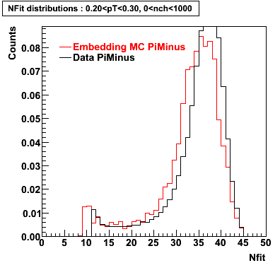 | 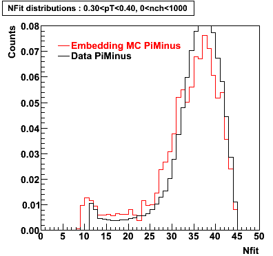 | 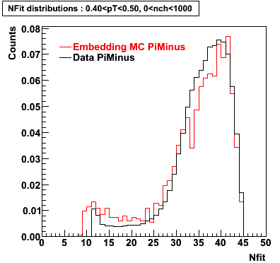 | 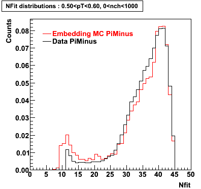 |
| 0.20 < pT < 0.30 | 0.30 < pT < 0.40 | 0.40 < pT < 0.50 | 0.50 < pT < 0.60 |
- Pi Plus
Pi Minus
|
||
|
||
|
||
|
||
|
Pi Plus
|
||
|
||
|
||
|
||
|
K Minus
|
||
|
||
|
||
|
||
|
K Plus
|
||
|
||
|
||
|
||
|
Proton
|
||
|
||
|
||
|
||
|
P bar
|
||
|
||
|
||
|
||
|
QA Plots Phi(Feb 2009)
QA P06ib (Phi->K +K)
This is the QA for P06ib (Phi- > KK). reconstruction on Global Tracks (Kaons)
1. dEdx
Reconstruction on Kaon Daugthers. Plot shows MOntecarlo tracks and Ghost Tracsks.
/P06ib_dedx_Phi(Ghost).gif)
2. DCA Distributions
An original 3D histogram had been created and filled with pT, Eta and DCA as the 3 coordinates. Projection on PtBins and EtaBins had been made to create this "matrix" of plots. (MonteCarlo and MuDst) (MuDst taken from pdsf > /eliza12/starprod/reco/cuProductionMinBias/ReversedFullField/P06ib/2005/022/st_physics_adc_6022048_raw*.MuDst.root)
Pt Bin array used : { 0.5, 0.6, 0.8, 1.0} (moves down) and
Eta Bin array : {0.2, 0.5, 0.8, 1.0} (moves to the right)
For the Error bars, i used the option hist->Sumw2();
/dca_eta_pt_phi.gif)
3. NFit Distributions
Similarly An Original 3D Histogram had been created with Pt, Eta and Nfit as coordinates. Respective projections had been made in the same pT and Eta Bins as the DCa distributions. (MonteCarlo and MuDst)
Pt Bin array used : { 0.5, 0.6, 0.8, 1.0} (moves down) and
Eta Bin array : {0.2, 0.5, 0.8, 1.0} (moves to the right)
For the Error bars, i used the option hist->Sumw2();
/nfit_eta_pt_phi.gif)
4. Delta Vertex
The following are the Delta Vertex ( Vertex Reconstructed - Vertex Embedded) plot for the 3 diiferent coordinates (x, y and z) (Cuts of vz =30 cm , NFitCut= 25 are applied)
/Delta_vertex_Phi.gif)
5. Z Vertex and X vs Y vertex
/vertex_Phi.gif)
6. Global Variables : Phi and Rapidity
/y_f_phi(1).gif)
/phi_f_phi.gif)
7. Pt
Embedded Phi meson with flat pt (black)and Reconstructed Kaon Daugther (red).
/pt_f_phi.gif)
8. Randomness Plots
The following plots, are to check the randomness of the input Monte Carlo (MC) tracks.
/mc_pt_y_Phi_K.gif)
/mc_y_phi_phi_K.gif)
QA plots Rho (February 16 2009)
QA P06ib (Rho->pi+pi)
This is the QA for P06ib (Rho- > pi+pi). reconstruction on Global Tracks (pions)
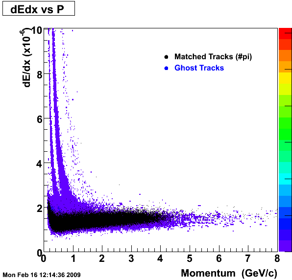
1. dEdx
Reconstruction on Pion Daugthers.
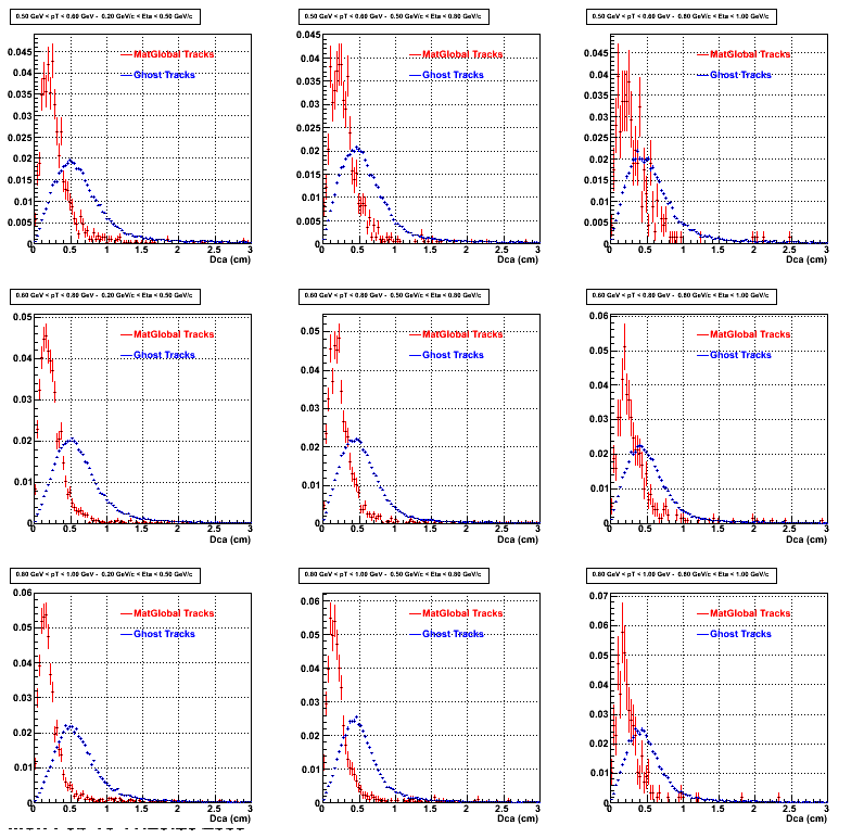
2. DCA Distributions
An original 3D histogram had been created and filled with pT, Eta and DCA as the 3 coordinates. Projection on PtBins and EtaBins had been made to create this "matrix" of plots.
Pt Bin array used : { 0.5, 0.6, 0.8, 1.0} (moves down) and
Eta Bin array : {0.2, 0.5, 0.8, 1.0} (moves to the right)
For the Error bars, i used the option hist->Sumw2();
2b. Compared with MuDst
.gif)
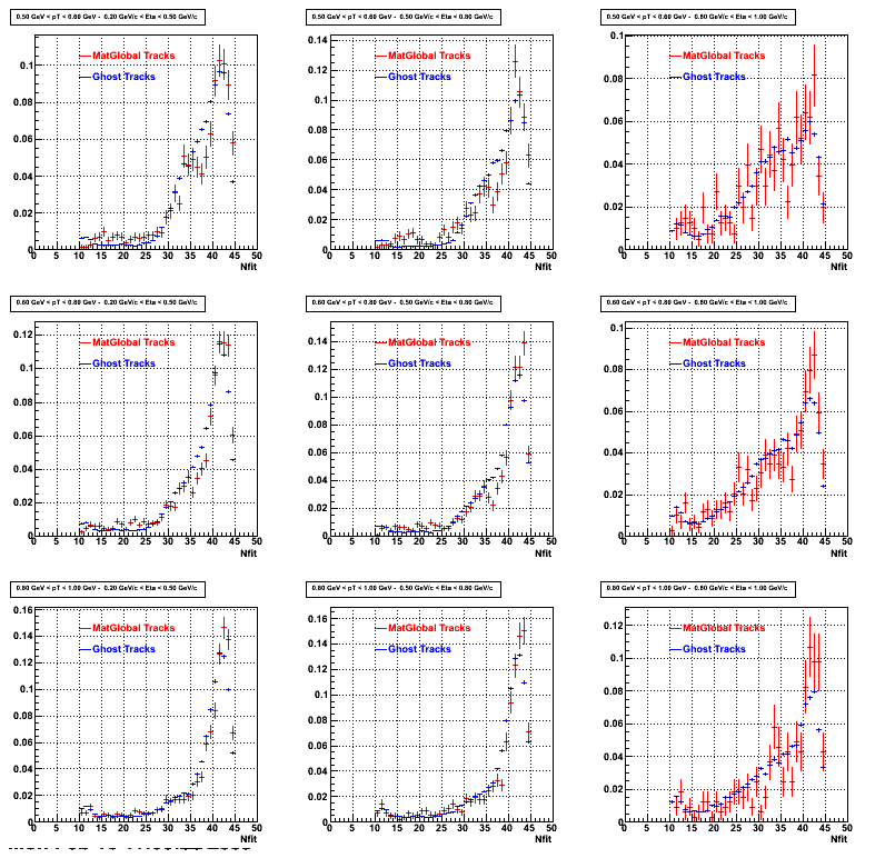
3. NFit Distributions
Similarly An Original 3D Histogram had been created with Pt, Eta and Nfit as coordinates. Respective projections had been made in the same pT and Eta Bins as the DCa distributions.
Pt Bin array used : { 0.5, 0.6, 0.8, 1.0} (moves down) and
Eta Bin array : {0.2, 0.5, 0.8, 1.0} (moves to the right)
For the Error bars, i used the option hist->Sumw2();
3b. Reconstructed compared with MuDsts
.gif)
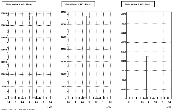
4. Delta Vertex
The following are the Delta Vertex ( Vertex Reconstructed - Vertex Embedded) plot for the 3 diiferent coordinates (x, y and z) (Cuts of vz =30 cm , NFitCut= 25 are applied)
5. Z Vertex and X vs Y vertex
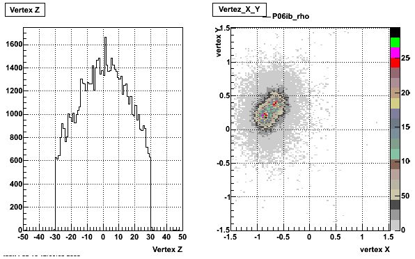
6. Global Variables : Phi and Rapidity
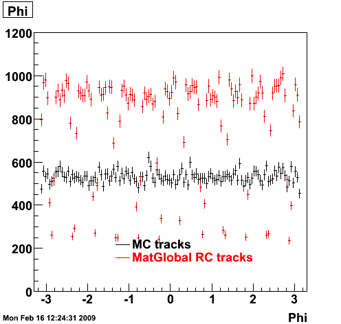
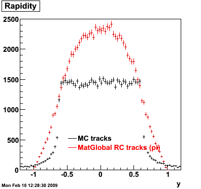
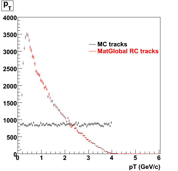
7. Pt
Embedded Rho meson with flat pt (black)and Recosntructed Pion (red).
8. Randomness Plots
The following plots, are to check the randomness of the input Monte Carlo (MC) tracks.
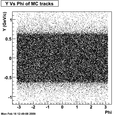
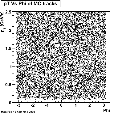
.gif)
QA plots Rho (October 21 2008)
Some QA plots for Rho:
MiniDst files are at PDSF under the path /eliza13/starprod/embedding/p06ib/MiniDst/rho_101/*.minimc.root
MuDst files are at PDSF under /eliza13/starprod/embedding/P06ib/MuDst/10*/*.MuDst.root Reconstruction had been done on PionPlus.
DCA and Nfit Distributions had been scaled by the Integral in different pt ranges
QAPlots_D0
Some QA Plots for D0 located under the path :
/eliza12/starprod/embedding/P06ib/D0_001_1216876386/*
/eliza12/starprod/embedding/P06ib/D0_002_1216876386/ -> Directory empty
Global pairs are used as reconstructed tracks. SOme quality tractst plotiing level were :
Vz Cut 30 cm ;
NfitCut : 25,
Ncommonhits : 10 ;
maxDca :1 cm ; Assuming D0- >pi + pi
P07ib
Test done on P07ib - Doing claibration on dE/dx |
 |
Fraction bla bla
 |
P05id
P05id Cu+Cu Embedding
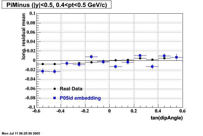
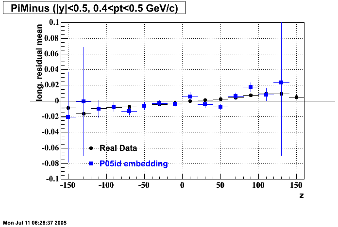
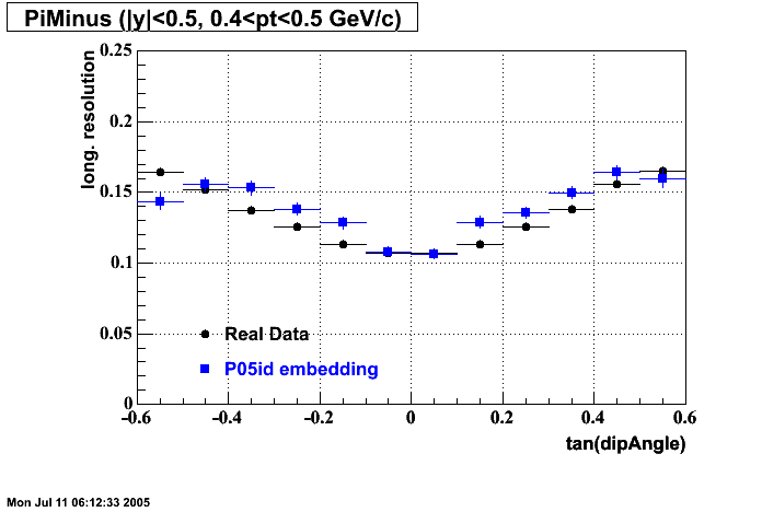
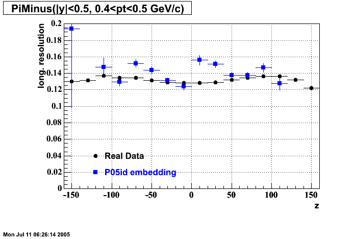
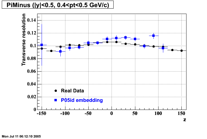
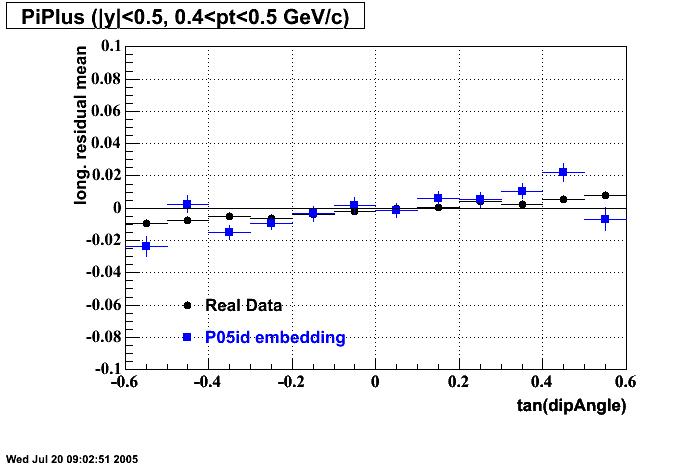
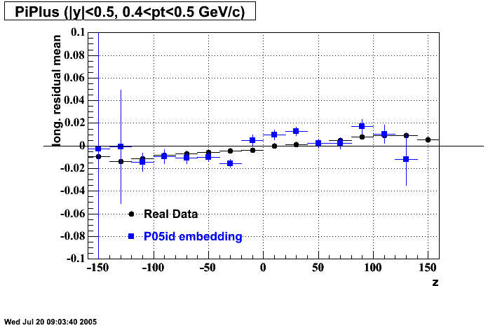
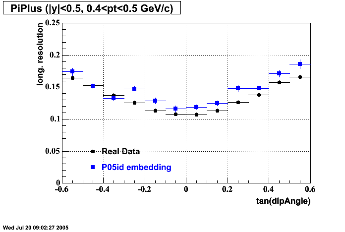
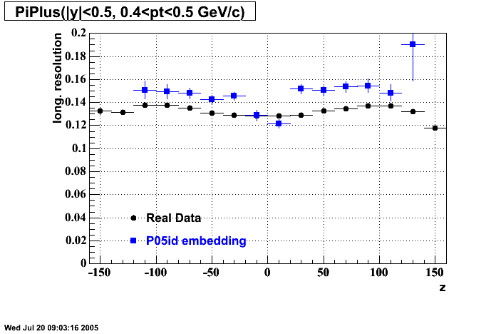
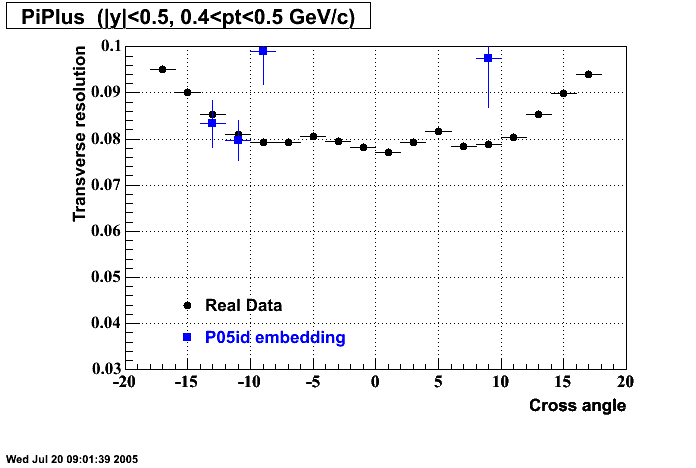
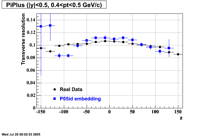
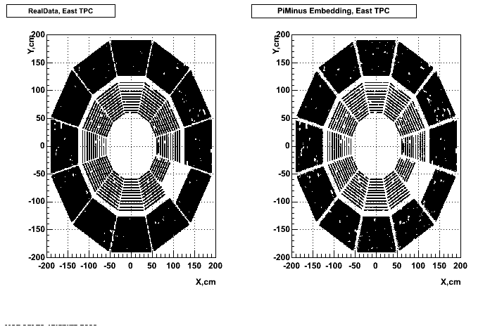
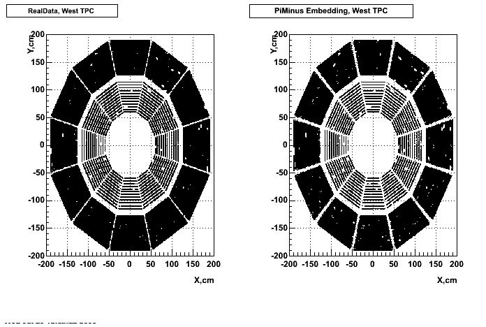
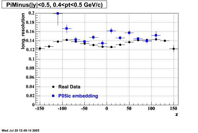
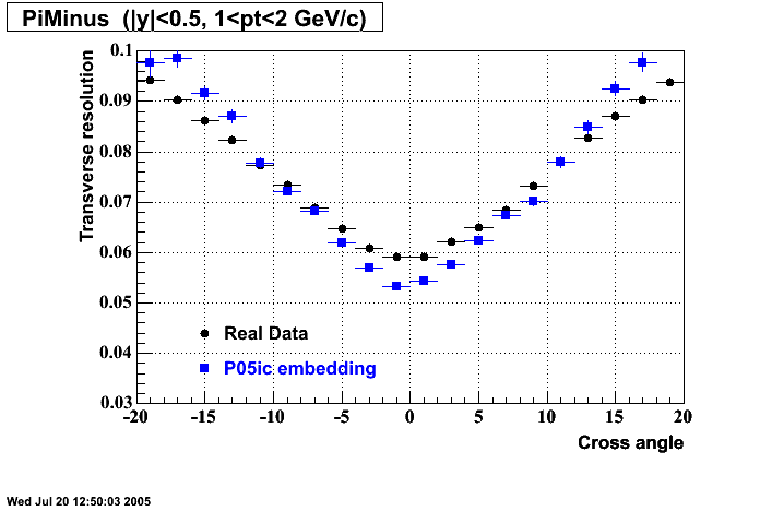
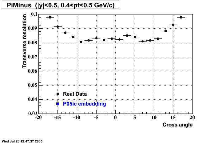
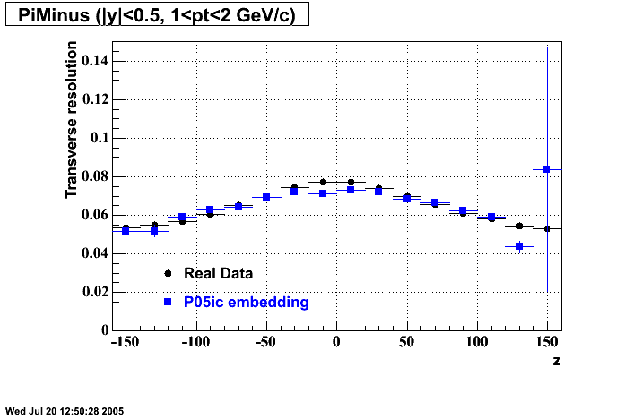
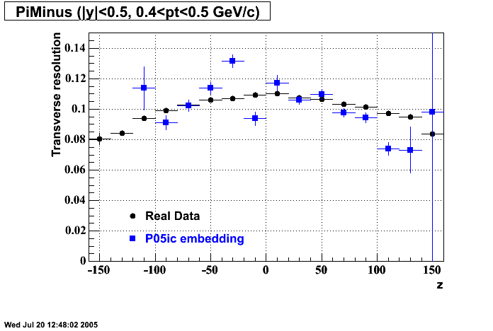
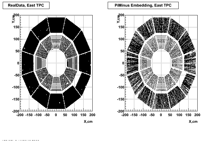
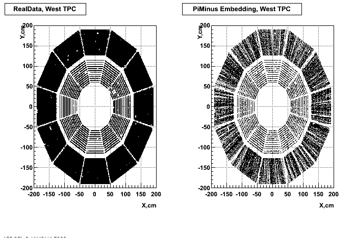
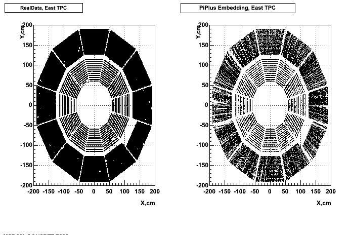
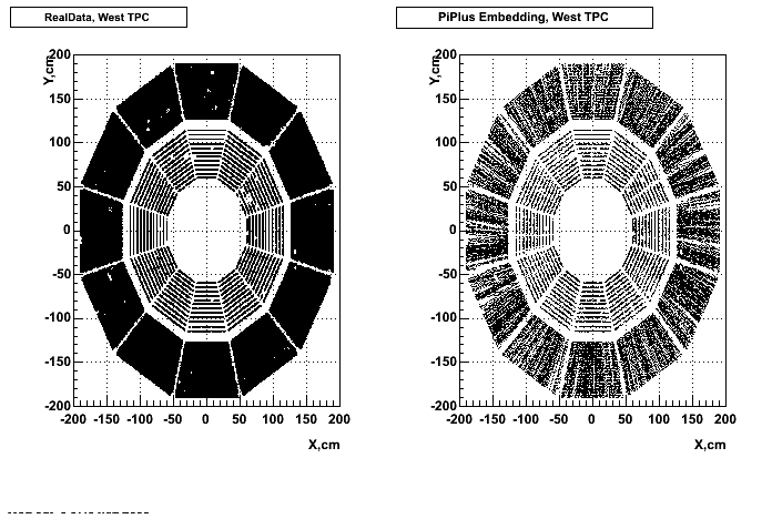
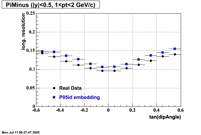
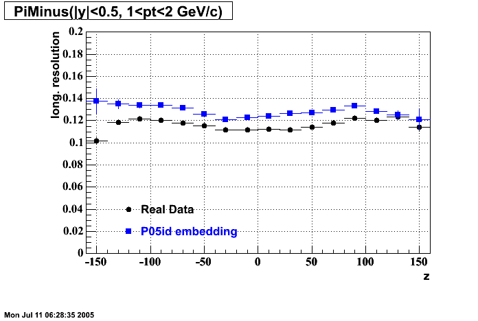
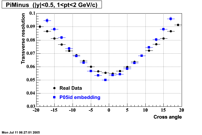
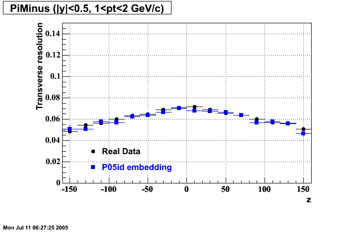
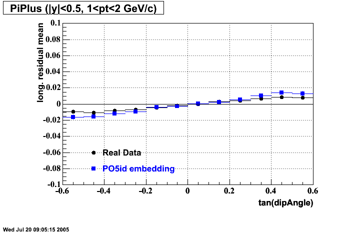
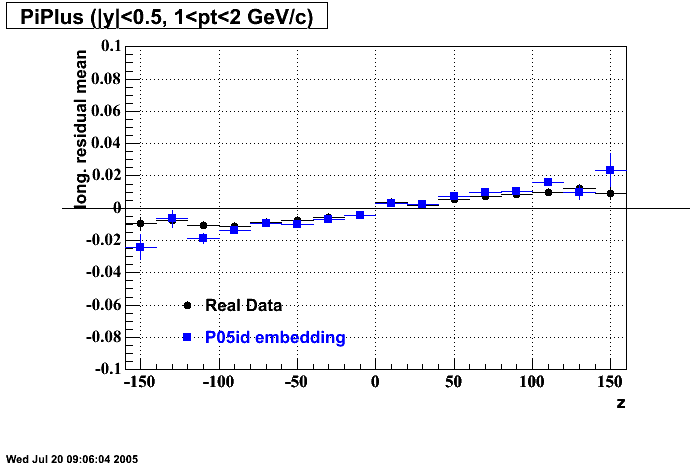
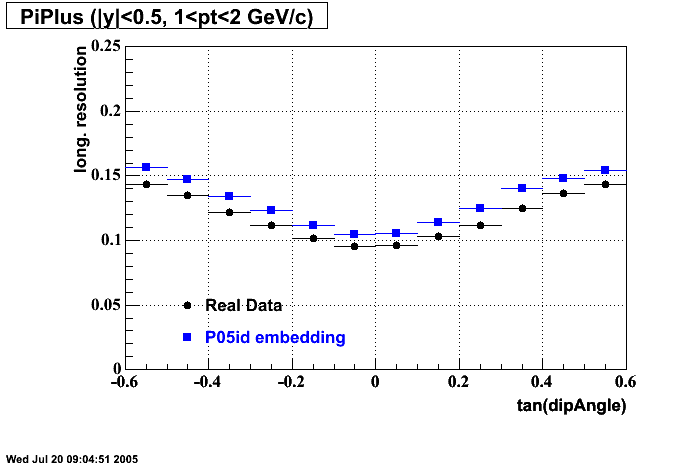
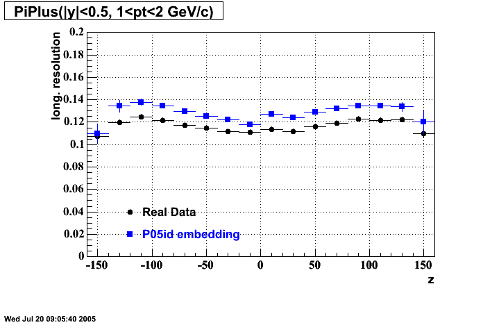
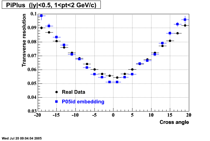
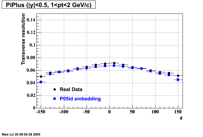
Hit level check-up : At the Hit level the results look in good agreement.
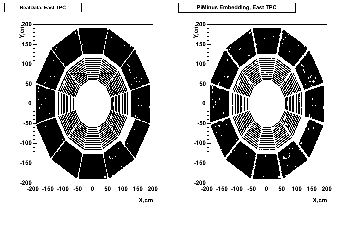
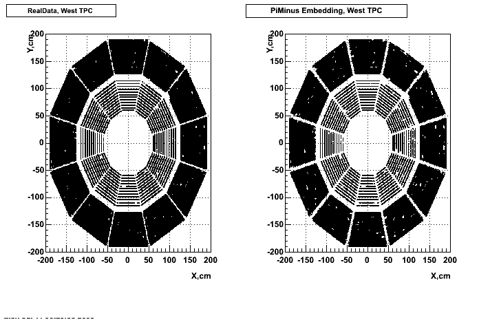
- Missing/Dead Areas (PiMinus): The next graphs show dead sectors for embeded data and real data as well.
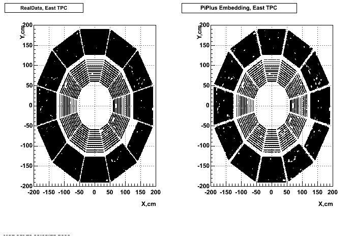
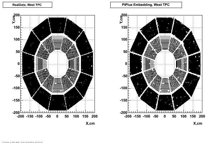
- Missing/Dead Areas (PiPlus)
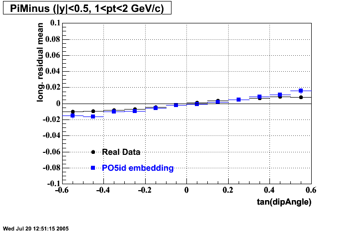
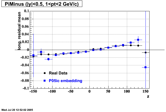
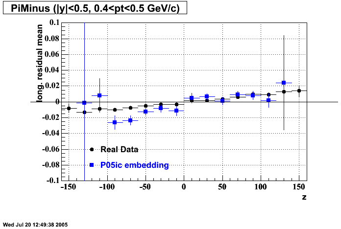
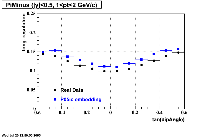
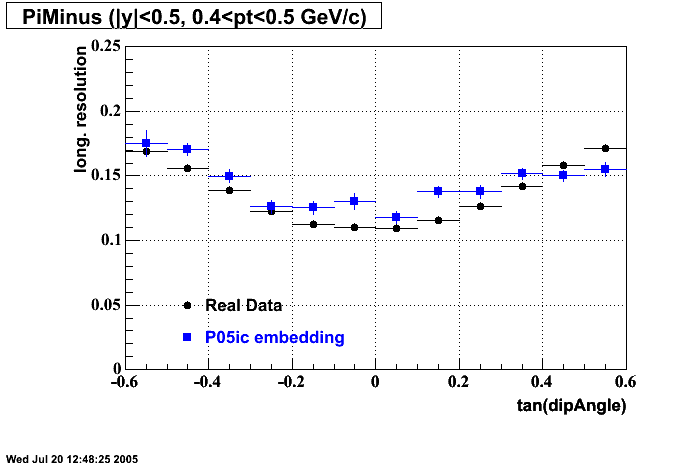
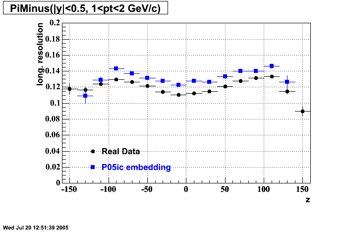
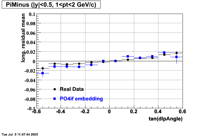
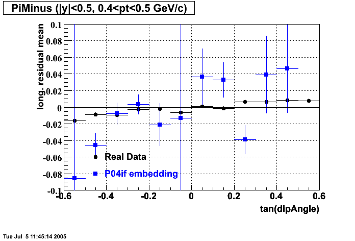
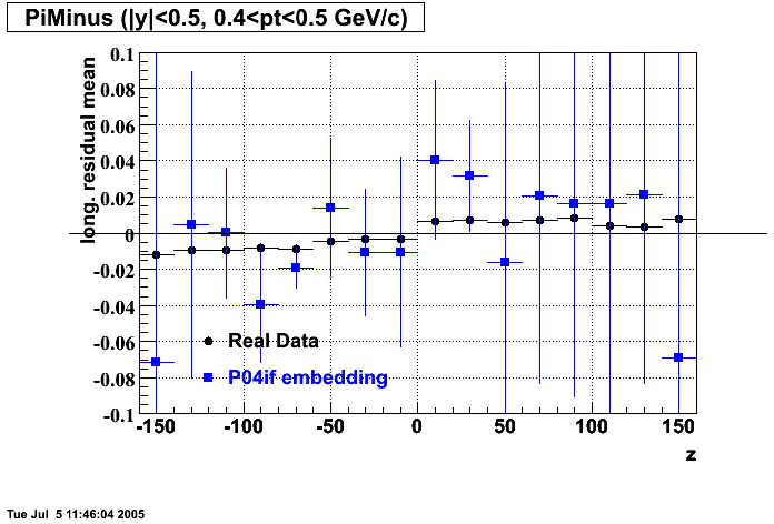
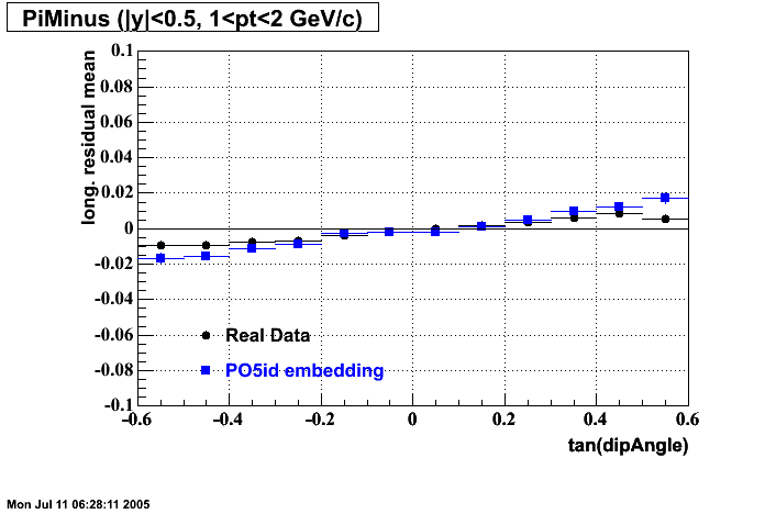
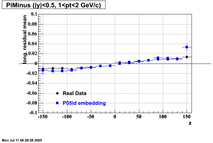
- Track Residuals PiMinus
- Track Residuals PiPlus
- dEdx Comparisons
 | |
 | |
 | |
 | |
 | |
 |
 | |
 | |
 | |
 | |
 | |
 |
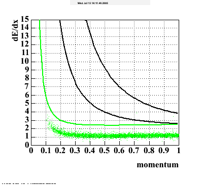
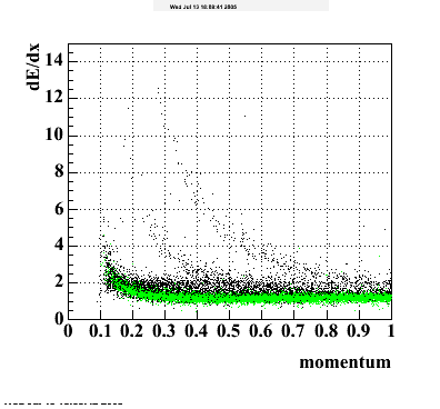
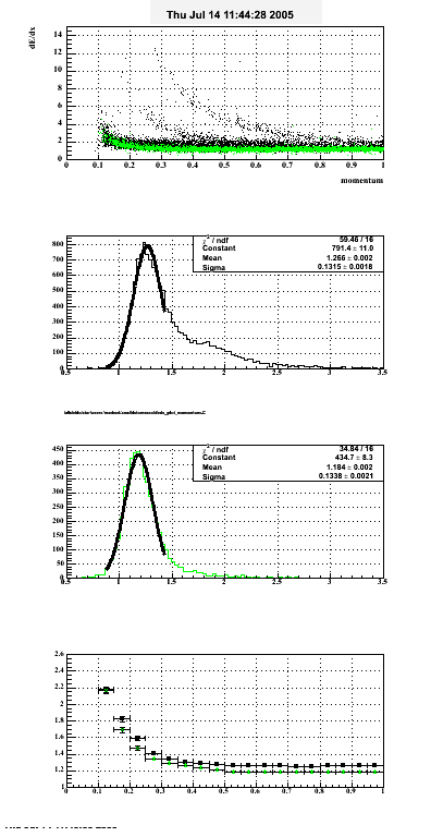
The following are results of dEdx calibration from embedding for Pi Minus. Graphs 1 and 2 are Dedx vs Momentum grapsh where Green dots are the MonteCarlo Tracks reconstructed from Embedding and Black dots are Data. In Graph Number 2, dots are Data and solid lines show Bichsel parametrisation with a factor of 1/2 offset. In the Last Graph a projection on dEdx axis is done and a MIP of 1.26 and 1.18 are shown.
 | |
 |
P08ic -Jpsi(Test)
QA P08ic J/Psi -> ee+
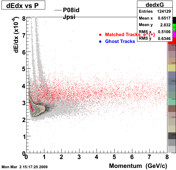
This is the QA for P08id (jPsi - > ee). Reconstructin on Global Tracks and just Electrons (Positrons).
1. dEdx
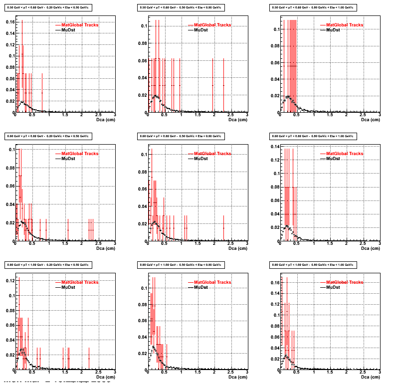
2. DCA Distributions
An original 3D histogram had been created and filled with pT, Eta and DCA as the 3 coordinates. Projection on PtBins and EtaBins had been made to create this "matrix" of plots.
Pt Bin array used : { 0.5, 0.6, 0.8, 1.0} (moves down) and
Eta Bin array : {0.2, 0.5, 0.8, 1.0} (moves to the right)
For the Error bars, i used the option hist->Sumw2();
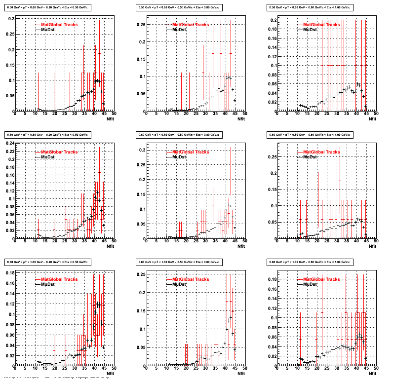
3. NFit Distributions
Similarly An Original 3D Histogram had been created with Pt, Eta and Nfit as coordinates. Respective projections had been made in the same pT and Eta Bins as the DCa distributions.
Pt Bin array used : { 0.5, 0.6, 0.8, 1.0} (moves down) and
Eta Bin array : {0.2, 0.5, 0.8, 1.0} (moves to the right)
For the Error bars, i used the option hist->Sumw2();
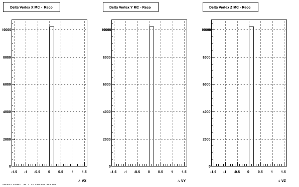
4. Delta Vertex
The following are the Delta Vertex ( Vertex Reconstructed - Vertex Embedded) plot for the 3 diiferent coordinates (x, y and z)
5. Z Vertex and X vs Y vertex
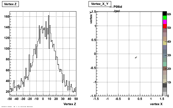
6. Global Variables : Phi and Rapidity
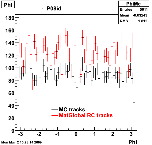
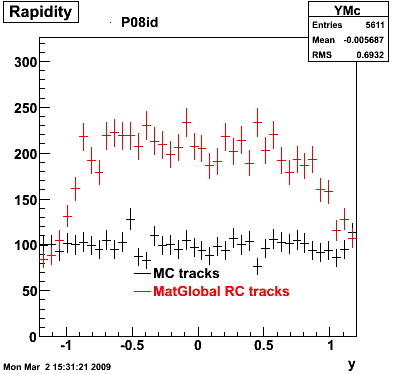
7. Pt
Embedded J/Psi with flat pt (black)and Recosntructed Electrons (red).

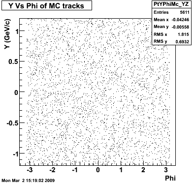
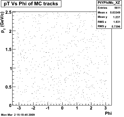
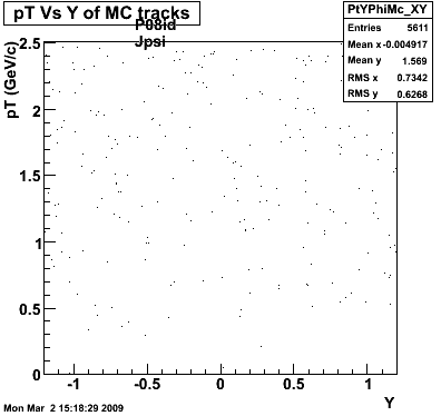
8. Randomness Plots
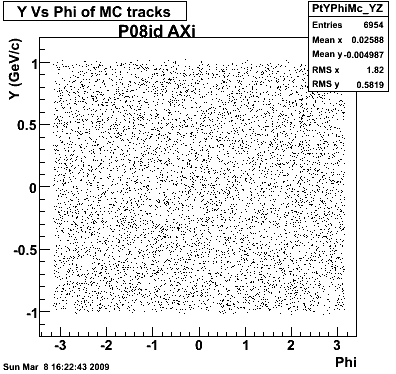
The following plots, are to check the randomness of the input Monte Carlo (MC) tracks.
P08id (AXi -> RecoPiPlus)
AXi-> Lamba + Pion + ->P + Pion - + Pion +
(03 08 2009)
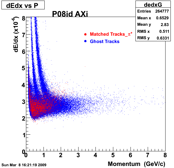
1. Dedx
2.Dca
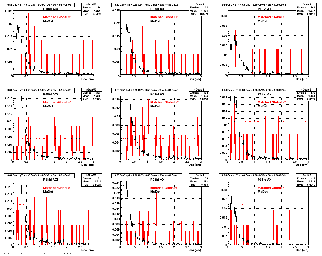
An original 3D histogram had been created and filled with pT, Eta and DCA as the 3 coordinates. Projection on PtBins and EtaBins had been made to create this "matrix" of plots.
Pt Bin array used : { 0.5, 0.6, 0.8, 1.0} (moves down) and
Eta Bin array : {0.2, 0.5, 0.8, 1.0} (moves to the right)
For the Error bars, i used the option hist->Sumw2();
3. Nfit
Similarly An Original 3D Histogram had been created with Pt, Eta and Nfit as coordinates. Respective projections had been made in the same pT and Eta Bins as the DCa distributions.
Pt Bin array used : { 0.5, 0.6, 0.8, 1.0} (moves down) and
Eta Bin array : {0.2, 0.5, 0.8, 1.0} (moves to the right)
For the Error bars, i used the option hist->Sumw2();

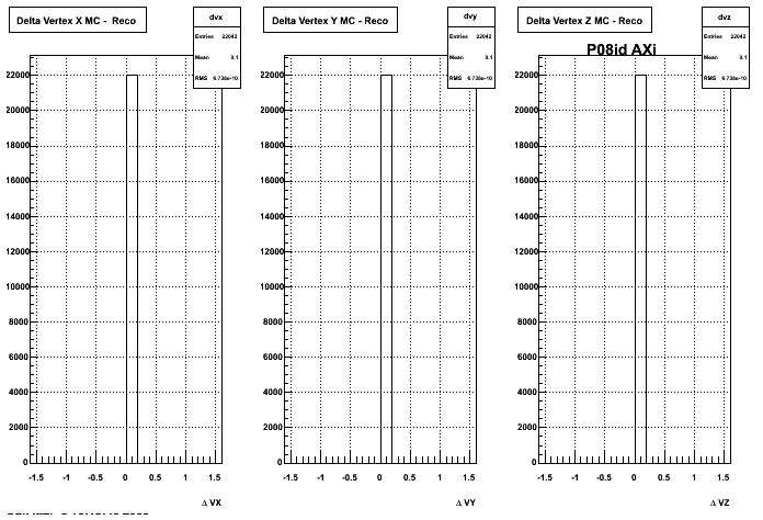
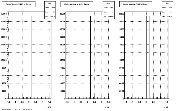
4. Delta Vertex
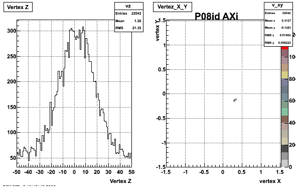
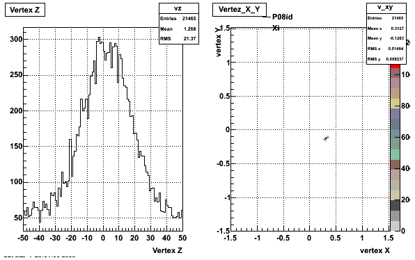
5. Z Vertex and X vs Y vertex
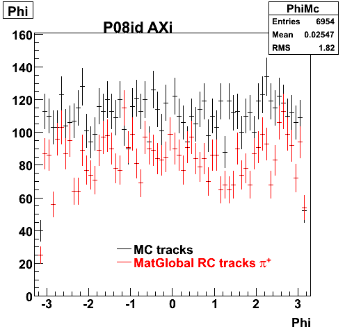
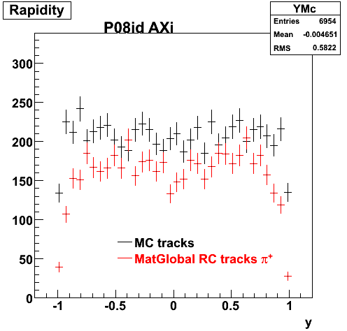
6. Global Variables : Phi and Rapidity
7. pt

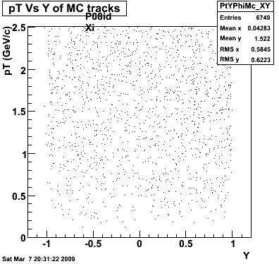
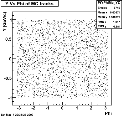
8. Randomness

P08id (Lambda->PK)
QA of Lambda Embedding with run 8 d+Au on PDSF (sample 15x)
Let's first check some event wise information. They look fine.

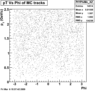
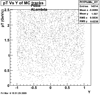
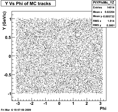
Then we check the randomness of the input Monte Carlo (MC) Lambda tracks. The 'phasespace' command in GSTAR is used for sampling the MC tracks. The input is supposed to be flat for pT within [0,8], Y [-1.5,1.5] and Phi [-Pi,Pi]. The 3 plots below show the randomness is OK for this sample. Please notice that Y is rapidity, not pseudo-rapidity.


Then we compare the dedx of reconstructed MC (matched) global tracks (i.e. the daughters of MC Lambda) to those of real (or ghost) tracks, to fix the scale factor. (scale factor = 1.38 ?)

Now we compare the nFitHits distribution of matched global tracks (i.e. the daughters of MC Lambda) and real tracks. The cuts are |eta|<1, nFitHits>25. For matched tracks, nCommonHits>10 cut is applied. From the left plot, we can see, the agreement of nHitFits is good for all pT ranges.

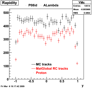
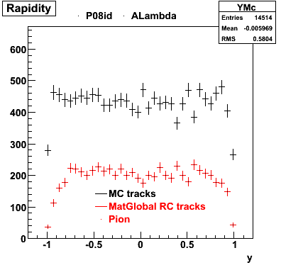
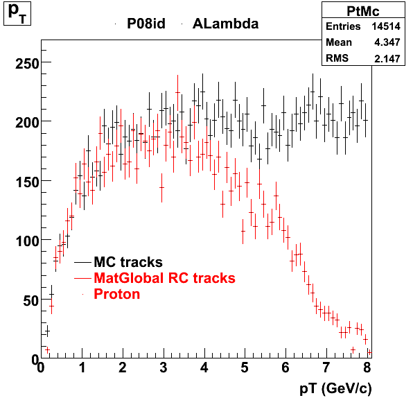
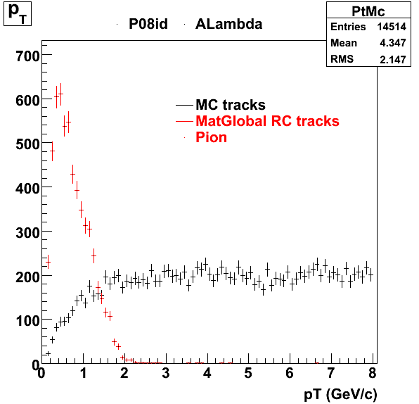
We check the pT, rapdity and Phi distributions of reconstruced (RC) Lambda and input (MC) Lambda. The cut for Lambda reconstruction is very loose. They look normal.


Here, we compare some cut variables from the reconstructed (RC) Lambda to those from real Lambda. Again, as you can see in these plots, the cuts are very loose for Lambda (contribution of background is estimated with rotation method, and has been subtracted). These plots are made for 8 pT bins (with rapidity cut |y|<0.75). The most obvious difference is in DCA of V0 to PV, especially for high pT bin.


P08id (Omega -> RecoPiMinus)
Omega-> Lamba + K - -> P + Pion - + K -
(03 08 2009)
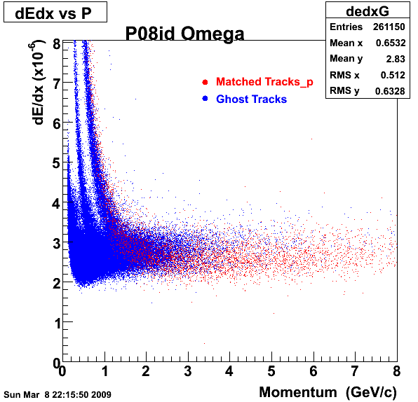
1. Dedx
Reconstruction on pion Minus and Proton Daugthers. 2 different plots are shown just for the sake of completenees.... Reconsructing on Kaon had very few statistics
| Reco PionMinus | Reco Proton |
 |  |
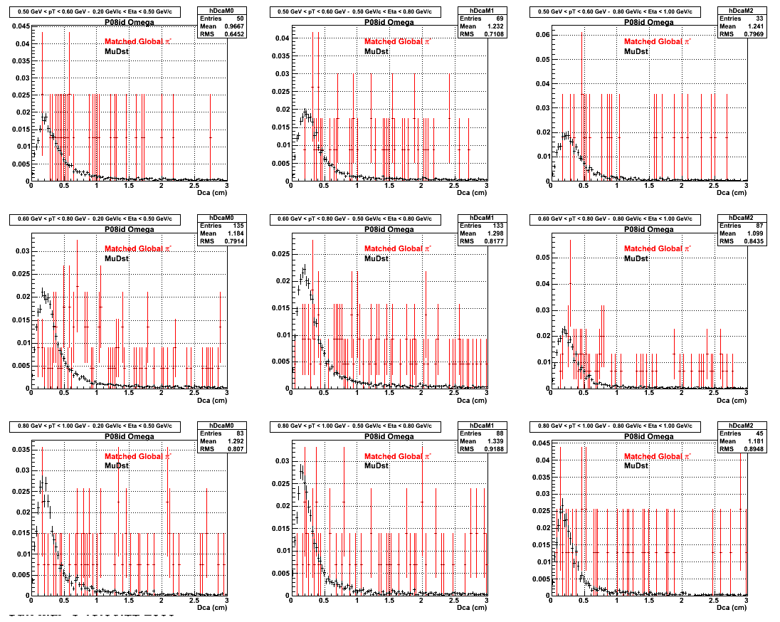
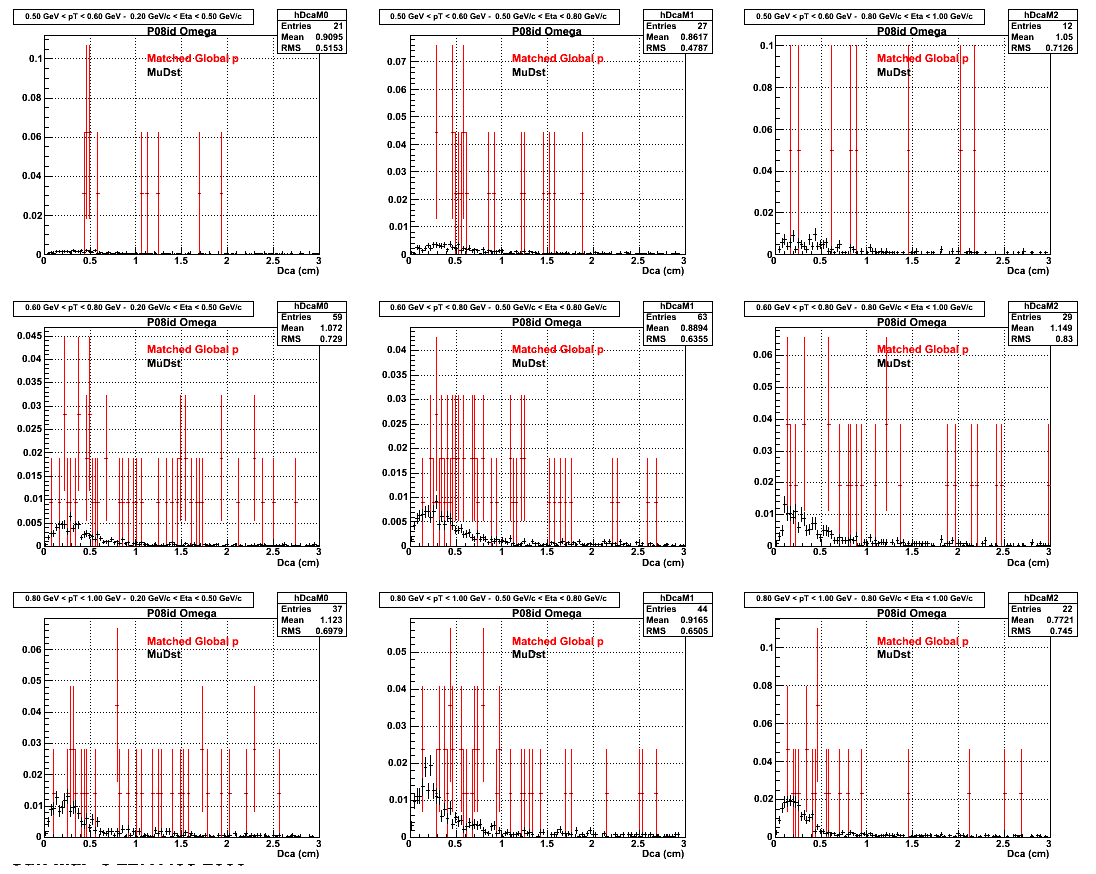
2.Dca
An original 3D histogram had been created and filled with pT, Eta and DCA as the 3 coordinates. Projection on PtBins and EtaBins had been made to create this "matrix" of plots.
Pt Bin array used : { 0.5, 0.6, 0.8, 1.0} (moves down) and
Eta Bin array : {0.2, 0.5, 0.8, 1.0} (moves to the right)
For the Error bars, i used the option hist->Sumw2();
*.Reconstructing on Pion
*. Reconstructing on Proton
3. Nfit
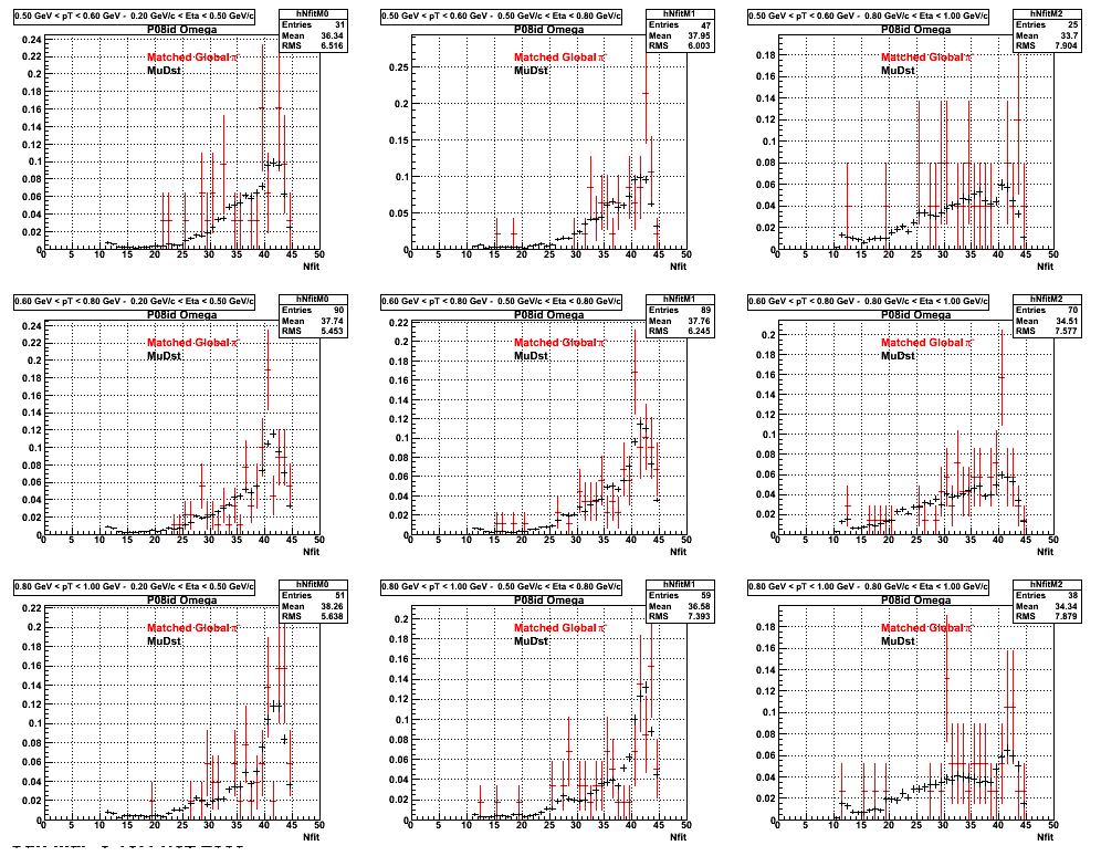
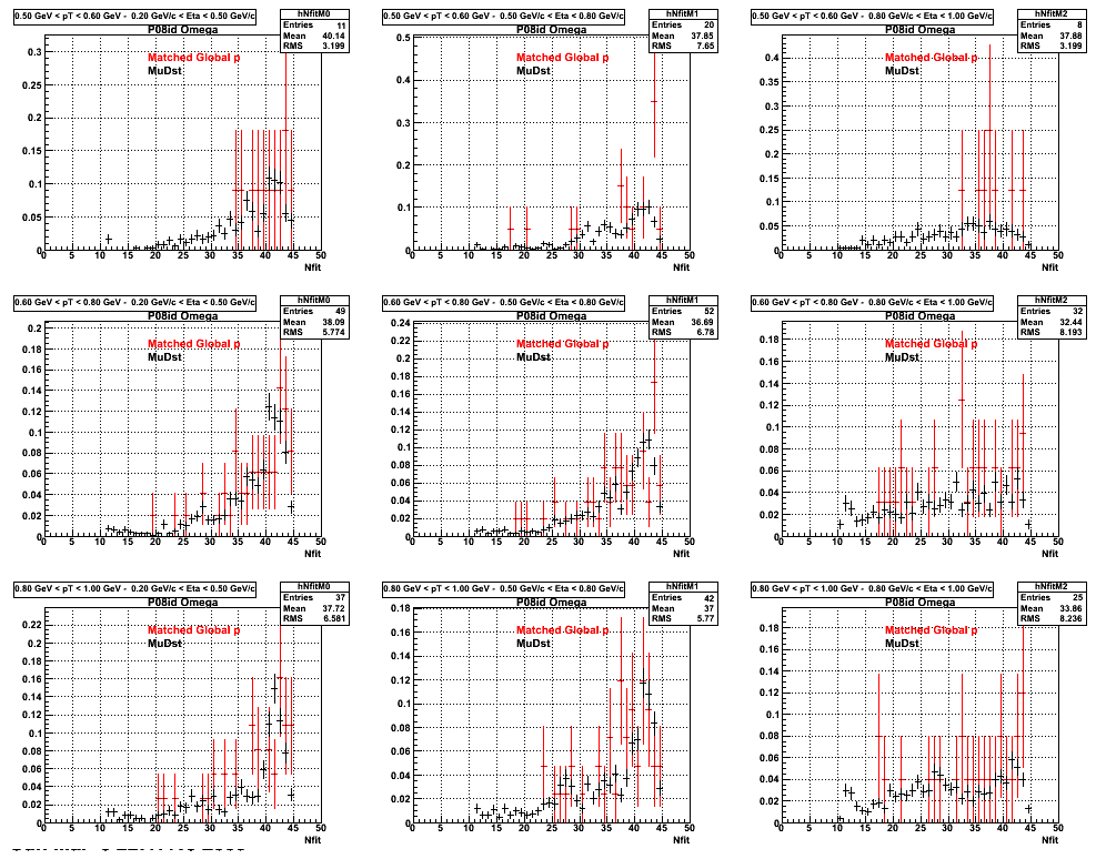
Similarly An Original 3D Histogram had been created with Pt, Eta and Nfit as coordinates. Respective projections had been made in the same pT and Eta Bins as the DCa distributions.
Pt Bin array used : { 0.5, 0.6, 0.8, 1.0} (moves down) and
Eta Bin array : {0.2, 0.5, 0.8, 1.0} (moves to the right)
For the Error bars, i used the option hist->Sumw2();
*. Reconstructing Pion
*. Reconstructing Proton
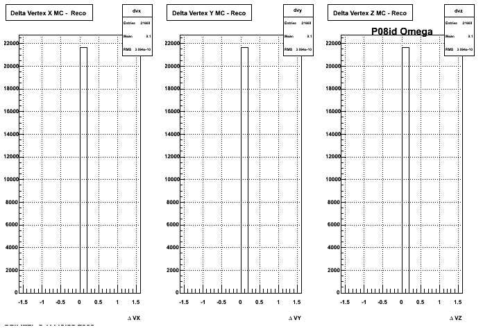
4. Delta Vertex
When reconstructed in Pion Minus and Proton it turns out to have the same ditreibutions so I just posted one of them
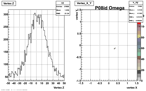
5. Z Vertex and X vs Y vertex
6. Global Variables : Phi and Rapidity
| Reco Pion | Reco Kaon |
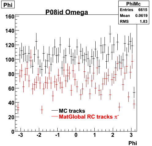 | 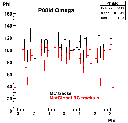 |
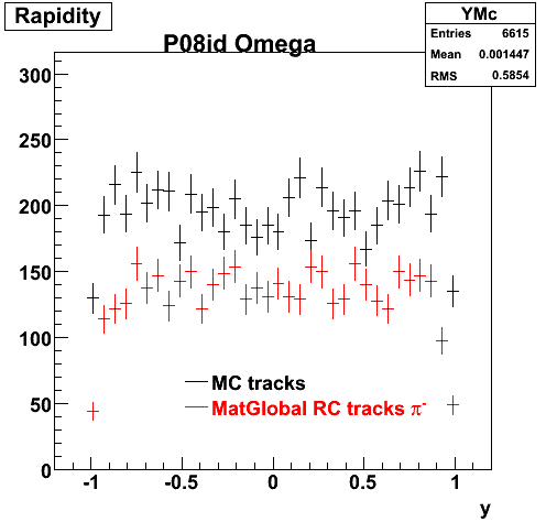 | 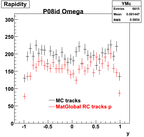 |
7. pt
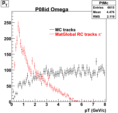
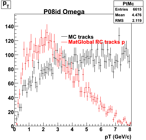
8. Randomness


P08id (phi ->KK) (March 05 2009)
QA Phi->KK (March 05 2009)
1. Dedx
Reconstruction on Kaon Daugthers. 2 different plots are shown just for the sake of completenees....
/Dedx_P08id_Phi_030509(Ghost.gif)
/Dedx_P08id_Phi_030509.gif)
2.Dca
An original 3D histogram had been created and filled with pT, Eta and DCA as the 3 coordinates. Projection on PtBins and EtaBins had been made to create this "matrix" of plots.
Pt Bin array used : { 0.5, 0.6, 0.8, 1.0} (moves down) and
Eta Bin array : {0.2, 0.5, 0.8, 1.0} (moves to the right)
For the Error bars, i used the option hist->Sumw2();
/DCA_eta_pt_P08id_Phi_030509.gif)
3. Nfit
Similarly An Original 3D Histogram had been created with Pt, Eta and Nfit as coordinates. Respective projections had been made in the same pT and Eta Bins as the DCa distributions.
Pt Bin array used : { 0.5, 0.6, 0.8, 1.0} (moves down) and
Eta Bin array : {0.2, 0.5, 0.8, 1.0} (moves to the right)
For the Error bars, i used the option hist->Sumw2();
/Nfit_eta_pt_P08id_Phi_030509.gif)
4. Delta Vertex
/DeltaVertex_P08id_Phi_030509.gif)
5. Z Vertex and X vs Y vertex
/Vertex_P08id_Phi_030509.gif)
6. Global Variables : Phi and Rapidity
/Phi_P08id_Phi_030509.gif)
/Rapidity_P08id_Phi_030509.gif)
7. pt
/pT_P08id_Phi_030509.gif)
8. Randomness
/Y_pT_P08id_Phi_030509.gif)
/pT_Phi_P08id_Phi_030509.gif)
P08id (phi ->KK)
QA P08id (Phi->KK)
This is the QA for P08id (phi - > KK). econstructin on Global Tracks and just Kaons. Macro from Xianglei used (I found the QA macro very familiar). scale factor of 1.38 applied.
1. dEdx
Reconstruction on Kaon Daugthers. 2 different plots are shown just to see how Montecarlo looks on top of the Ghost Tracks
/dedx_f1_38(1).gif)
/dedx_v2_f1_38.gif)
2. DCA Distributions
An original 3D histogram had been created and filled with pT, Eta and DCA as the 3 coordinates. Projection on PtBins and EtaBins had been made to create this "matrix" of plots.
Pt Bin array used : { 0.5, 0.6, 0.8, 1.0} (moves down) and
Eta Bin array : {0.2, 0.5, 0.8, 1.0} (moves to the right)
For the Error bars, i used the option hist->Sumw2();
/dca_eta_pt(1).gif)
3. NFit Distributions
Similarly An Original 3D Histogram had been created with Pt, Eta and Nfit as coordinates. Respective projections had been made in the same pT and Eta Bins as the DCa distributions.
Pt Bin array used : { 0.5, 0.6, 0.8, 1.0} (moves down) and
Eta Bin array : {0.2, 0.5, 0.8, 1.0} (moves to the right)
For the Error bars, i used the option hist->Sumw2();
/nfit_eta_pt(1).gif)
4. Delta Vertex
The following are the Delta Vertex ( Vertex Reconstructed - Vertex Embedded) plot for the 3 diiferent coordinates (x, y and z)
/DeltaVX.gif)
/DeltaVY.gif)
/DeltaVZ.gif)
5. Z Vertex and X vs Y vertex
/vertex_1_38.gif)
6. Global Variables : Phi and Rapidity
/phi_f1_38.gif)
/y_f1_38.gif)
7. Pt
Embedded Phi meson with flat pt (black)and Recosntructed Kaons (red).
/pt_f1_38.gif)
8. Randomness Plots
The following plots, are to check the randomness of the input Monte Carlo (MC) tracks.
/mc_pt_phi.gif)
/mc_pt_y.gif)
P08id(ALambda -> P, Pion)
QA ALambda->P, pi (03 08 2009)
1. Dedx
Reconstruction on Proton and Pion Daugthers. 2 different plots are shown just for the sake of completenees....
| Reco Proton | Reco Pion |
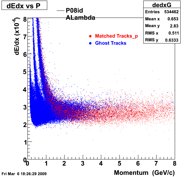 | 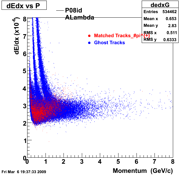 |
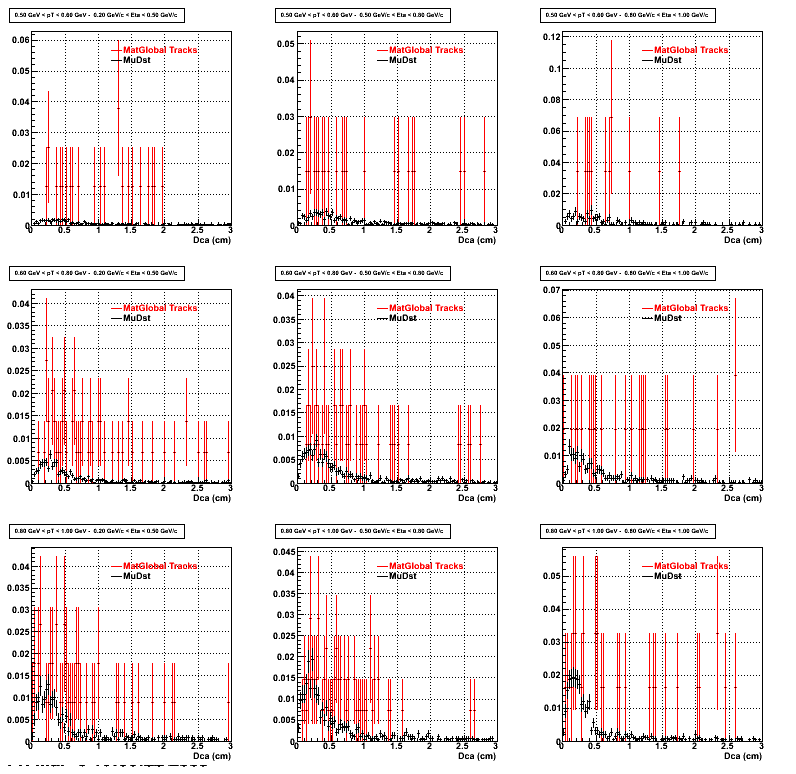
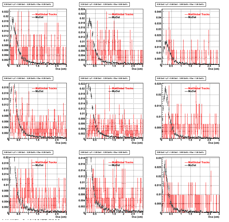
2.Dca
An original 3D histogram had been created and filled with pT, Eta and DCA as the 3 coordinates. Projection on PtBins and EtaBins had been made to create this "matrix" of plots.
Pt Bin array used : { 0.5, 0.6, 0.8, 1.0} (moves down) and
Eta Bin array : {0.2, 0.5, 0.8, 1.0} (moves to the right)
For the Error bars, i used the option hist->Sumw2();
*.Reconstructing on Proton
*. Reconstructing on Pion
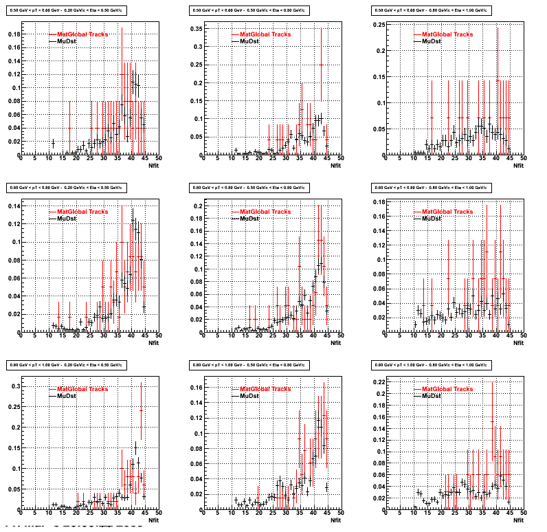
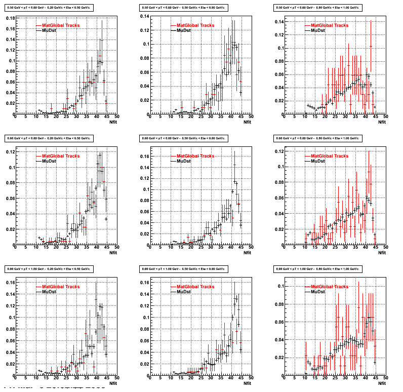
3. Nfit
Similarly An Original 3D Histogram had been created with Pt, Eta and Nfit as coordinates. Respective projections had been made in the same pT and Eta Bins as the DCa distributions.
Pt Bin array used : { 0.5, 0.6, 0.8, 1.0} (moves down) and
Eta Bin array : {0.2, 0.5, 0.8, 1.0} (moves to the right)
For the Error bars, i used the option hist->Sumw2();
*. Reconstructing Proton
*. Reconstructing Pion
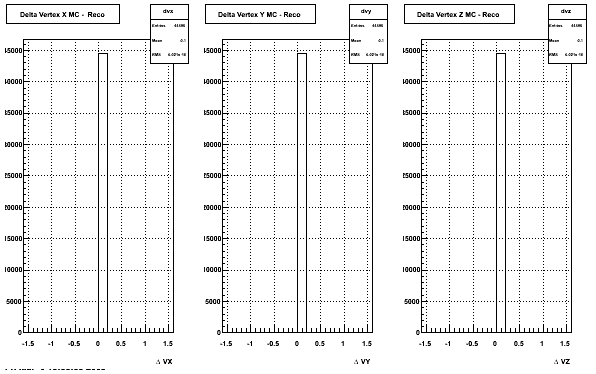
4. Delta Vertex
When reconstructed in Proton and pions it turns out to have the same ditreibutions so I just posted one of them
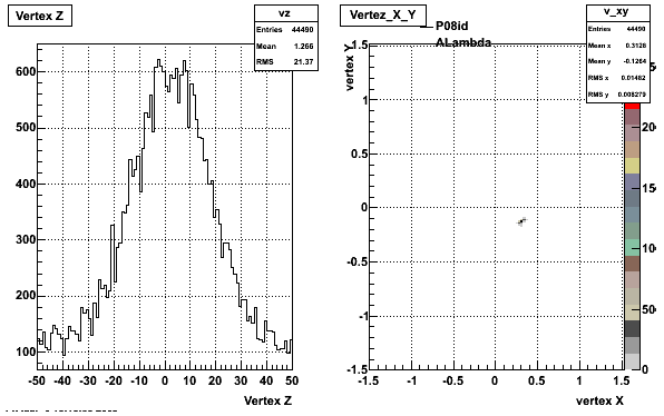
5. Z Vertex and X vs Y vertex
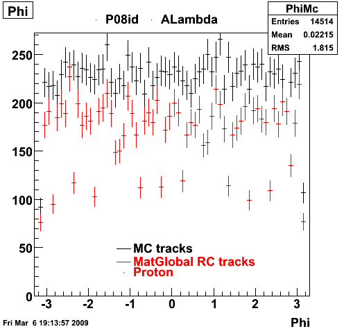
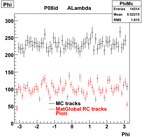
6. Global Variables : Phi and Rapidity
| Reco Proton | Reco Pion |
 |  |
 |  |
7. pt
8. Randomness
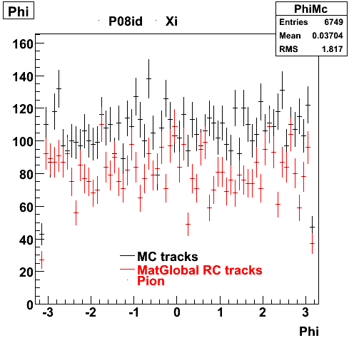
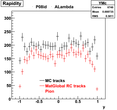
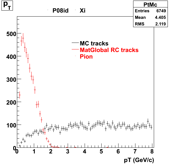
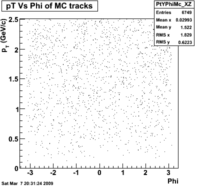
P08id(Xi -> Reco(PiMinus)
Xi-> Lamba + Pion - ->P + Pion - + Pion -
(03 08 2009)
1. Dedx
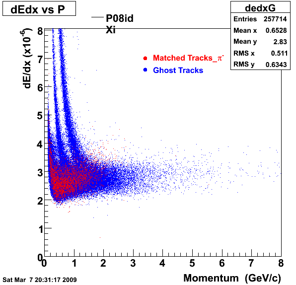
Reconstruction on PI Minus
2.Dca
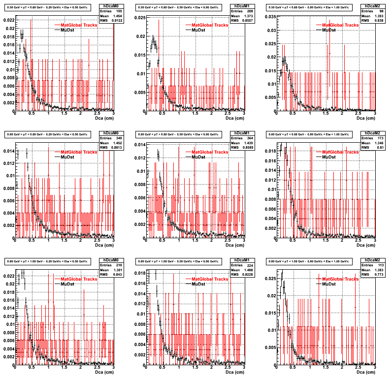
An original 3D histogram had been created and filled with pT, Eta and DCA as the 3 coordinates. Projection on PtBins and EtaBins had been made to create this "matrix" of plots.
Pt Bin array used : { 0.5, 0.6, 0.8, 1.0} (moves down) and
Eta Bin array : {0.2, 0.5, 0.8, 1.0} (moves to the right)
For the Error bars, i used the option hist->Sumw2();
3. Nfit
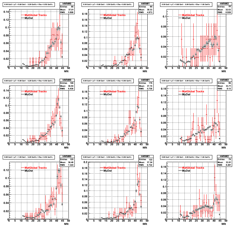
Similarly An Original 3D Histogram had been created with Pt, Eta and Nfit as coordinates. Respective projections had been made in the same pT and Eta Bins as the DCa distributions.
Pt Bin array used : { 0.5, 0.6, 0.8, 1.0} (moves down) and
Eta Bin array : {0.2, 0.5, 0.8, 1.0} (moves to the right)
For the Error bars, i used the option hist->Sumw2();
4. Delta Vertex
5. Z Vertex and X vs Y vertex
6. Global Variables : Phi and Rapidity
7. pt
8. Randomness
Phi->KK(Mar 12)
Please find the QA plots here
The data looks good.
Reconstructed phi meson has small rapidity dependence.
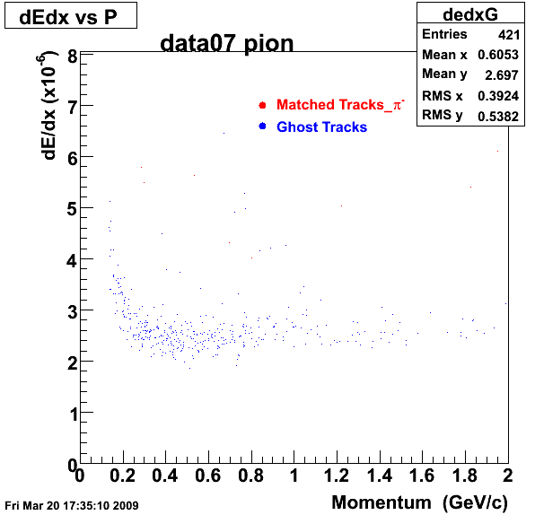
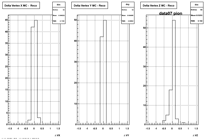
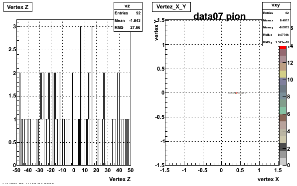
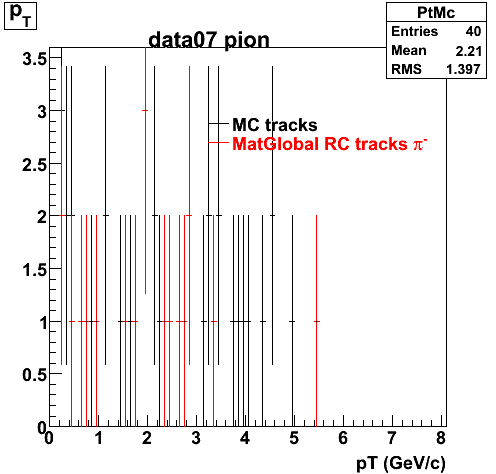
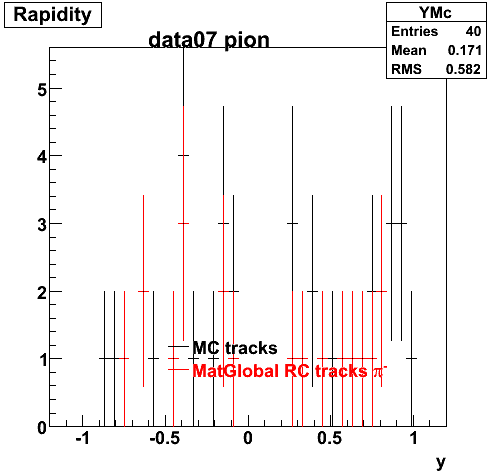
Yuri_Test_PionMinus_032009
![]() QA PionMinus
QA PionMinus
P04if
-
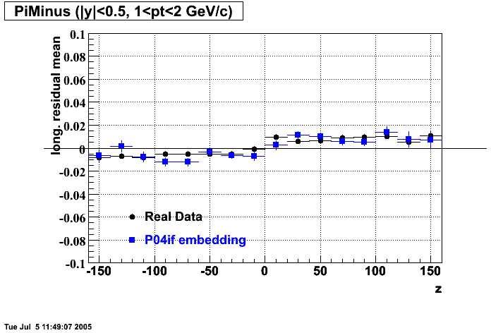
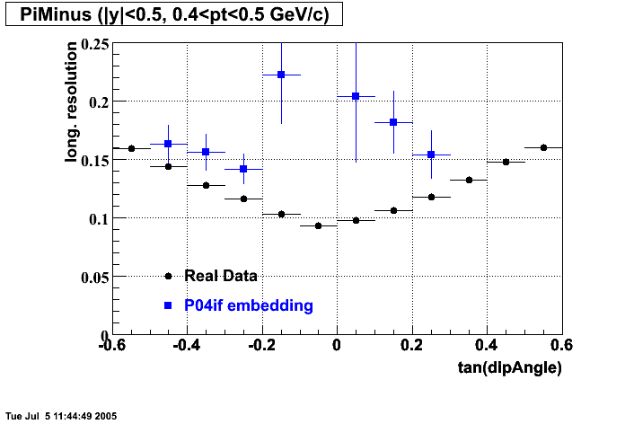
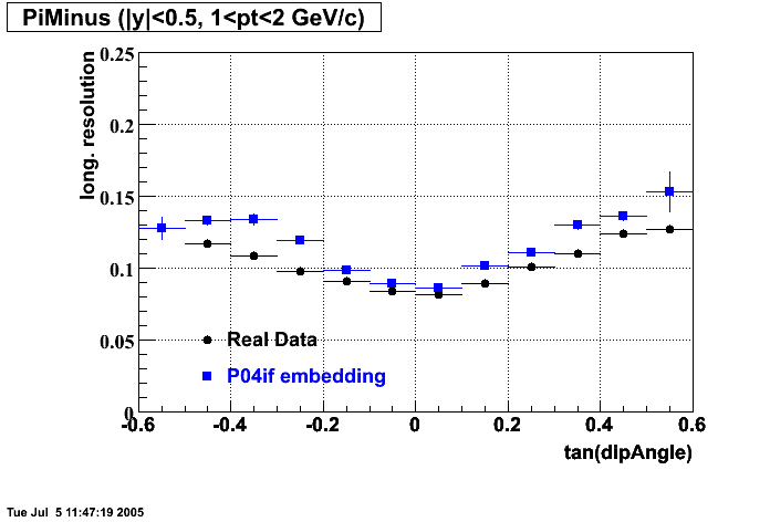
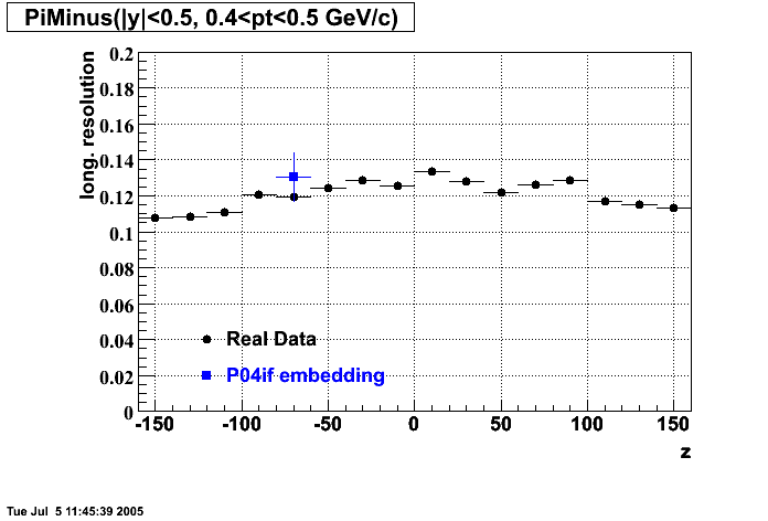
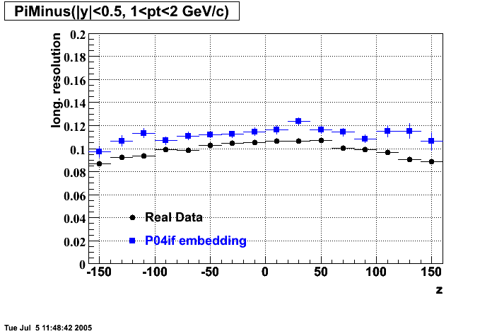
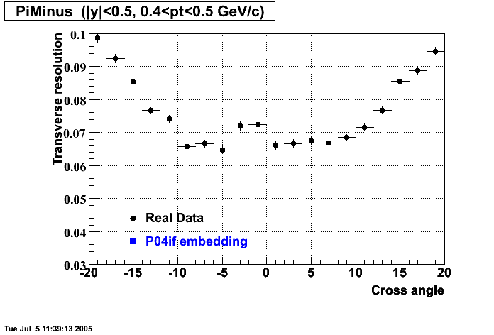
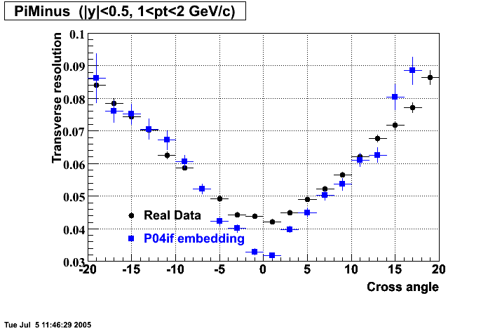
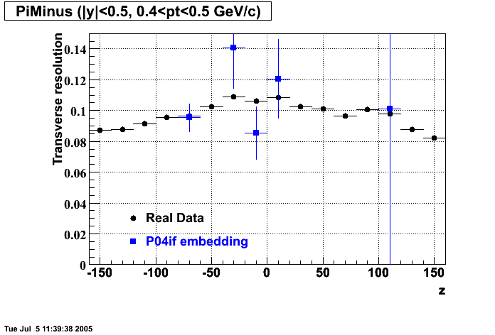
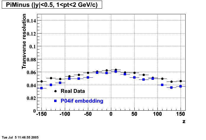
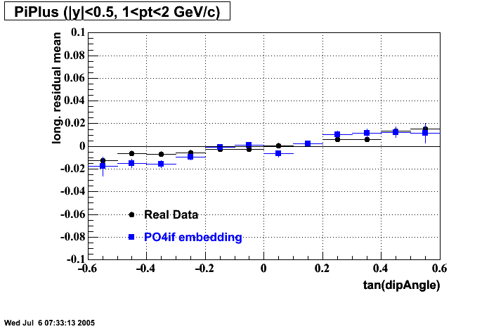
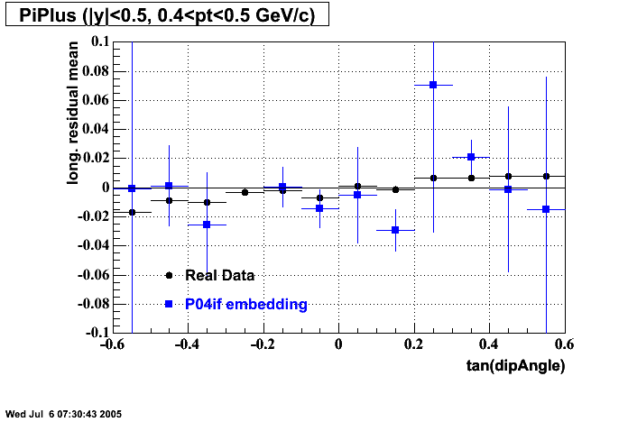
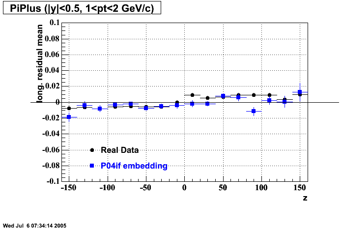
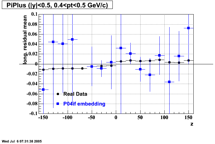
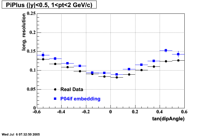
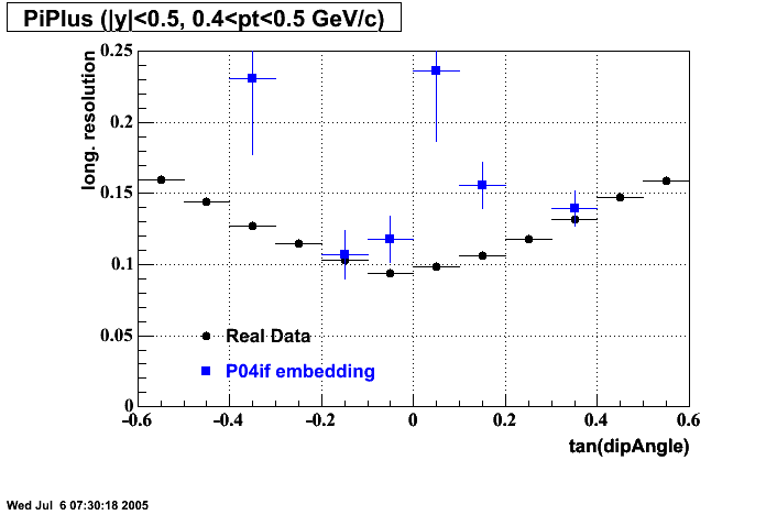
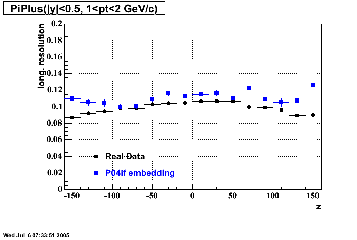
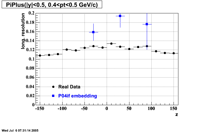
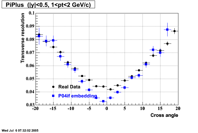
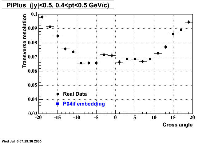
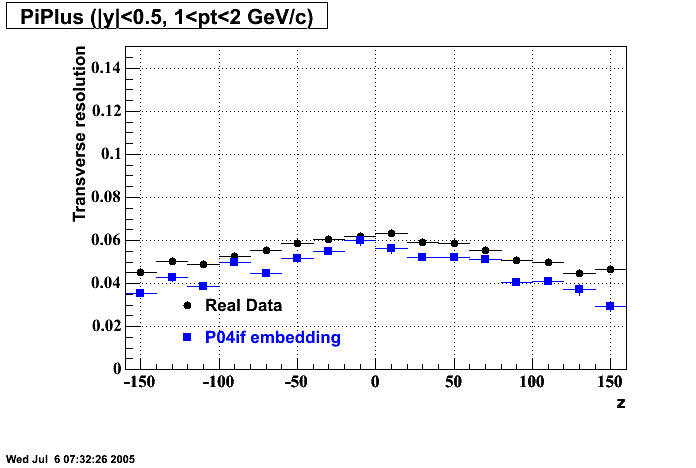
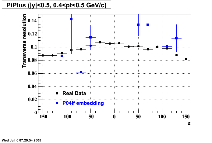
Hit level check-up:
Previous results - May 2002
This document is intended to provide all the information available for previous productions such that results for Quality Control studies and Productions Cross checks. Part of quality control studies include identification of missing/dead detector areas, distance of closest approach distributions (dca), and fit points distributions(Nfit). As part of production cross checks, some results in centrality dependance and efficiency are shown
Quality Control
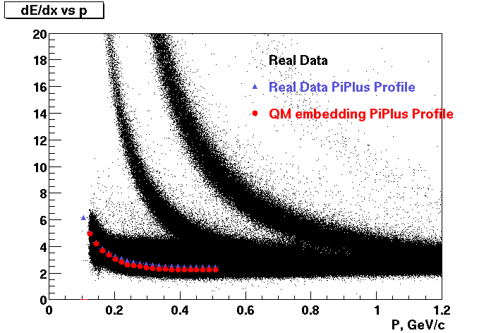
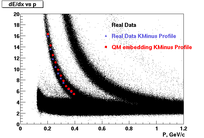
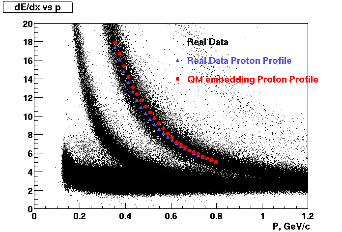
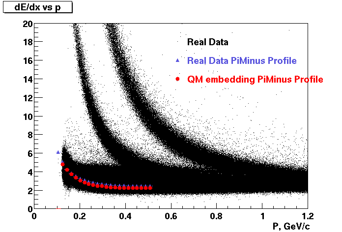
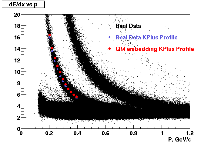
These are dedx vs P graphs. All of them show reasonable agreement with data.(Done on May 2002)
| Pi Minus | K Minus | Proton |
| Pi Plus | K Plus | P Bar |
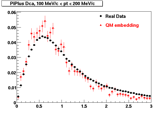
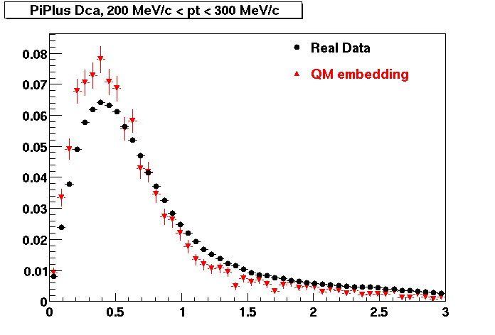
PI PLUS. In the following dca distributions some discrepancy is shown. Due to secondaries?
| Peripheral 0.1 GeV/c < pT < 0.2 Gev/c | MinBias 0.2 GeV/c < pT < 0.3 Gev/c | Central 0.3 GeV/c <pT < 0.4 GeV/c |
PI MINUS. Some discrepancy is shown. Due to secondaries?
| Peripheral 0.1 GeV/c < pT < 0.2 Gev/c | MinBias 0.2 GeV/c < pT < 0.3 Gev/c | Central 0.3 GeV/c <pT < 0.4 GeV/c |
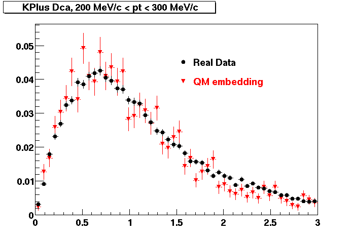
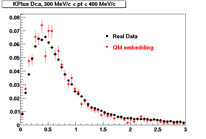
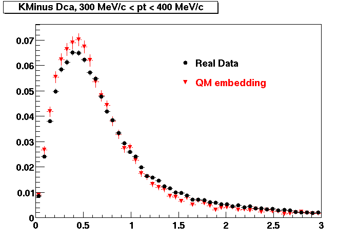
K PLUS. In the following dca distributions Good agreement with data is shown.
| Peripheral 0.1 GeV/c < pT < 0.2 Gev/c | MinBias 0.2 GeV/c < pT < 0.3 Gev/c | Central 0.3 GeV/c <pT < 0.4 GeV/c |
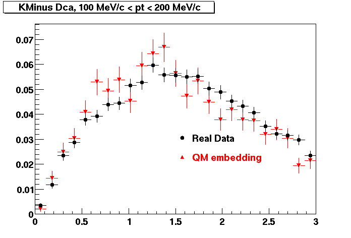
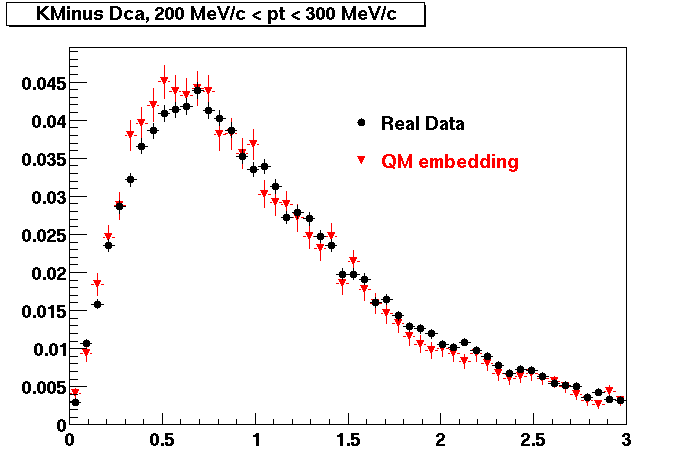
K MINUS. In the following dca distributions Good agreement with data is shown.
| Peripheral 0.1 GeV/c < pT < 0.2 Gev/c | MinBias 0.2 GeV/c < pT < 0.3 Gev/c | Central 0.3 GeV/c <pT < 0.4 GeV/c |
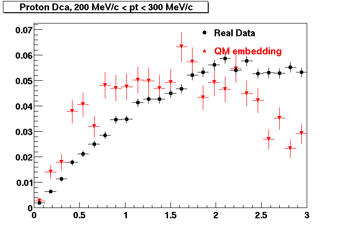
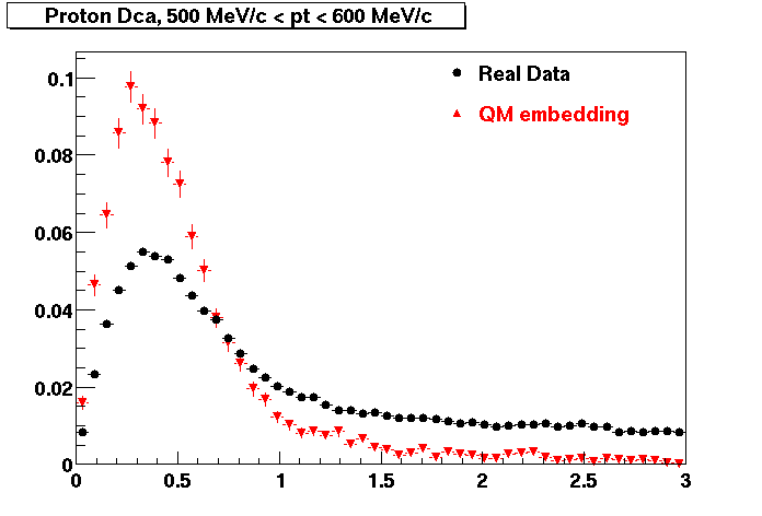
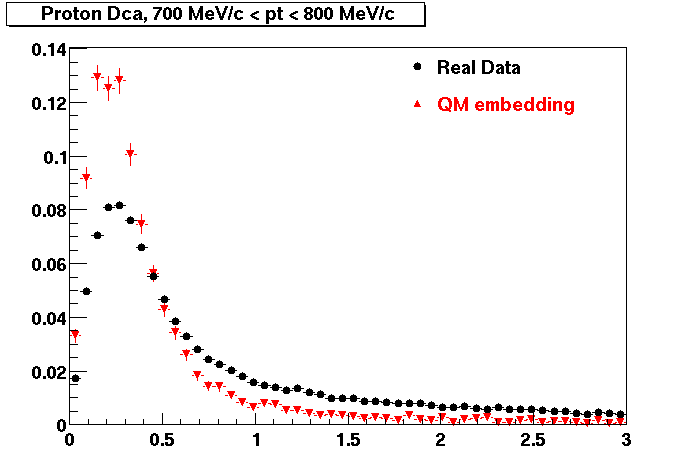
PROTON. The real data Dca distribution is wider, especially at low pT -> Most likely due to secondary tracks in the sample. A tail from background protons dominating distribution at low pt can be clearly seen. Expected deviation from the primary MC tracks.
| Peripheral 0.2 GeV/c < pT < 0.3 Gev/c | MinBias 0.5 GeV/c < pT < 0.6 Gev/c | Central 0.7 GeV/c <pT < 0.8 GeV/c |
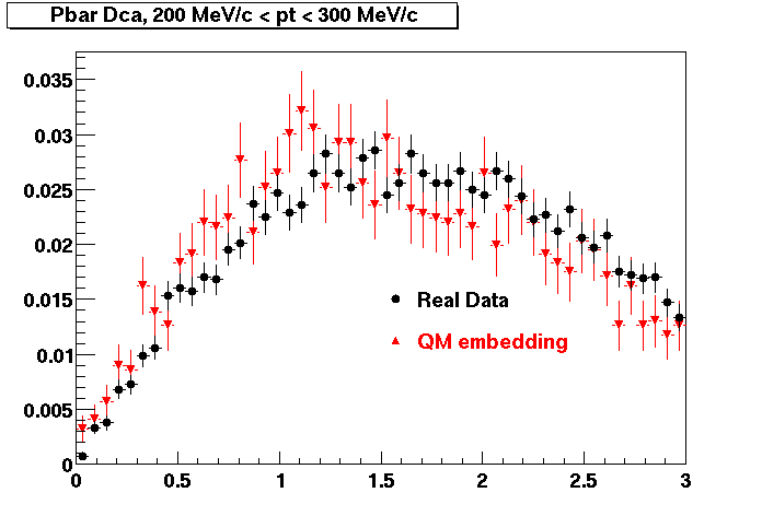
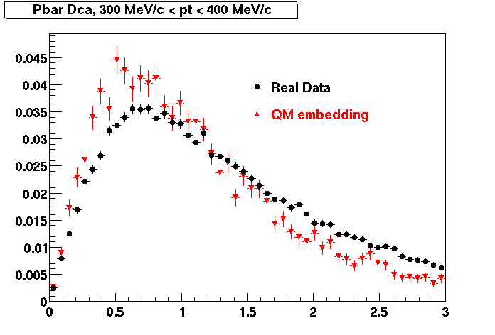
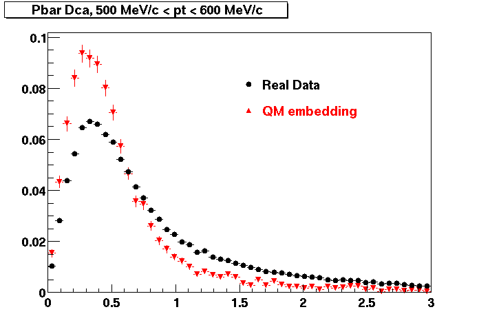
Pbar. The real data Dca distribution is wider, especially at low pT -> Most likely due to secondary tracks in the sample.
| Peripheral 0.2 GeV/c < pT < 0.3 Gev/c | MinBias 0.3 eV/c < pT < 0.4 Gev/c | Central 0.5 GeV/c <pT < 0.6 GeV/c |
PI PLUS. Good agreement with data is shown.
| Peripheral 0.1 GeV/c < pT < 0.2 Gev/c | MinBias 0.2 GeV/c < pT < 0.3 Gev/c | Central 0.3 GeV/c <pT < 0.4 GeV/c |
PI MINUS. Good agreement with data is shown.
| Peripheral 0.1 GeV/c < pT < 0.2 Gev/c | Peripheral 0.2 GeV/c < pT < 0.3 Gev/c | Peripheral 0.3 GeV/c < pT < 0.4 Gev/c |
K PLUS. Good agreement with data is shown.
| Peripheral 0.1 GeV/c < pT < 0.2 Gev/c | MinBias 0.2 GeV/c < pT < 0.3 Gev/c | Central 0.3 GeV/c <pT < 0.4 GeV/c |
K MINUS. Good agreement with data is shown.
| Peripheral 0.1 GeV/c < pT < 0.2 Gev/c | Peripheral 0.2 GeV/c < pT < 0.3 Gev/c | Peripheral 0.3 GeV/c < pT < 0.4 Gev/c |
PROTON. Good agreement with data is shown.
| Peripheral 0.2 GeV/c < pT < 0.3 Gev/c | Peripheral 0.3 GeV/c < pT < 0.4 Gev/c | Peripheral 0.5 GeV/c < pT < 0.6 Gev/c |
Pbar. Good agreement with data is shown.
| Peripheral 0.2 GeV/c < pT < 0.3 Gev/c | Peripheral 0.3 GeV/c < pT < 0.4 Gev/c | Peripheral 0.5 GeV/c < pT < 0.6 Gev/c |
