Charged Pions
Charged pion analysis
Run 5
2005 Charged Pion Data / Simulation Comparison
Motivation:Estimates of trigger bias systematic error are derived from simulation. This page compares yields obtained from data and simulation to test the validity of the PYTHIA event generator and our detector geometry model.
Conditions:
- Simulation DB timestamp: dbMk->SetDateTime(20050506,214129). I pick this table up from the DB, rather than from Dave's private directory. Dave changed the timestamps on the files in his directory, so the two files do not match. It turns out that in this case they only differ by one tower (4580), and this tower's status is != 1 in both tables, so there is effectively no difference.
- Data runlist: I use a version of the jet golden run list containing 690 runs. I have heard there is an updated version floating around, but I have yet to get my hands on it
- Simulation files obtained from production P05ih, including larger event samples from Lidia's recent email (http://www.star.bnl.gov/HyperNews-star/protected/get/starsoft/6437.html) but excluding the 2_3, 45_55, and 55_65 GeV samples.
- This is strictly a charged hadron comparison, there is no dE/dx PID cut. The dE/dx dsitributions in simulation are way off.
- Cuts: nFitPoints>25 && |dca|<1. && |eta|<1. && |vz|<60. && pt>2. Also for data I require good spin info and relative luminosity information (these conditions are mostly subsumed by the runlist requirement).
Combine PYTHIA partonic pt samples by filling histograms with weight = sample_weight/nevents, using sample_weights
- 3_4 = 1.287;
- 4_5 = 3.117e-1;
- 5_7 = 1.360e-1;
- 7_9 = 2.305e-2;
- 9_11 = 5.494e-3;
- 11_15 = 2.228e-3;
- 15_25 = 3.895e-4;
- 25_35 = 1.016e-5;
- above_35 = 5.299e-7;
Results:
At the moment I've just linked the raw PDFs at the bottom of the page. The index in the title indicates the charge of the particle being studied. The plots are perhaps a bit hard to follow without labels (next on the list), so here's a guide. Page 1 has pt distributions for the triggers in the order listed above. Pages 2-6 are eta distributions, with each page devoted to a single trigger, again in the order given above. The first plot on each page is integrated over all pt, and then the remaining plots separate the distribution into 1 GeV pt slices. Pages 7-11 repeat this structure for phi, and 12-16 do the same for the z-vertex distributions.
Conclusions:
The agreement between data and simulation appears to be me to be quite good across the board. The jet-patch triggers are particularly well-modeled. A few notes:
- The HT2 pt distributions (page 1, third plot on top row) look funny in simulation. What's with the spike at 6 GeV in the h- plot?
- HT2 eta distribution on the east side for h+ (page 4) has spikes.
- Phi looks good to me
- Vertex distributions for calo triggers in simulation are awfully choppy, but overall the agreement seems OK.
Average Partonic Pt Carried by Charged Pions
Here's a fragmentation study looking at the ratio of reconstructed charged pion p_{T} and the event partonic p_{T} in PYTHIA. Cuts are
- fabs(mcVertexZ()) < 60
- fabs(vertexZ()) < 60
- geantId() == 8 or 9 (charged pions)
- fabs(etaPr()) < 1
- fabs(dcaGl()) < 1
- fitPts() > 25

Error bars are just the errors on the mean partonic p_{T} in each reconstructed pion p_{T} bin. Next step is to look at the jet simulations to come up with a plot that is more directly comparable to a real data measurement.
BBC Vertex
This is a study of 2005 data conducted in March 2006. Ported to Drupal from MIT Athena in October 2007
Goal: Quantify the relationship between the z-vertex position and the bbc timebin for each event.
Procedure: Plot z-vertex as a function of trigger and bbc timebin. Also, plot distributions of bbc timebins for each run to examine stability. Exclude runs<=6119039 as a result. Fit each vertex distribution with a gaussian and extract mean, sigma. Plots are linked at the bottom of the page. See in particular page 8 of run_plots.pdf, which shows the change from 8 bit to 4 bit onlineTimeDifference values.
Timebin 12 had zero counts for each trigger. Summaries of the means and sigmas:
| m | 4 | 5 | 6 | 7 | 8 | 9 | 10 | 11 | 12 |
| mb | 101.7 | 124.1 | 56.3 | 22.72 | -7.835 | -38.89 | -80.48 | -135.6 | - |
| ht1 | 81.09 | 111.8 | 50.75 | 16.88 | -13.49 | -44.57 | -89.36 | -182.8 | - |
| ht2 | 79.86 | 107.2 | 48.93 | 15.76 | -14.27 | -45.17 | -89.76 | -176.7 | - |
| jp1 | 101.3 | 139.3 | 54.8 | 17.68 | -12.95 | -44.05 | -92.4 | -176 | - |
| jp2 | 99.49 | 128.5 | 51.58 | 15.77 | -14.29 | -45.5 | -94.1 | -192.2 | - |
| s | 4 | 5 | 6 | 7 | 8 | 9 | 10 | 11 | 12 |
| mb | 68.85 | 67.48 | 40.4 | 34.26 | 33.31 | 35.91 | 49.32 | 76.29 | - |
| ht1 | 68.99 | 70.9 | 43.06 | 34.71 | 32.49 | 34.86 | 47.42 | 79.98 | - |
| ht2 | 67.64 | 70.13 | 43.06 | 34.76 | 32.55 | 34.98 | 47.26 | 78.22 | - |
| jp1 | 76.49 | 79.85 | 45.44 | 35.6 | 32.56 | 35.34 | 49.69 | 78.1 | - |
| jp2 | 76.18 | 78.01 | 45.73 | 35.79 | 32.87 | 35.68 | 49.37 | 81.21 | - |
Conclusions: Hank started the timebin lookup table on day 119, so this explains the continuous distributions from earlier runs. In theory one could just use integer division by 32 to get binned results before this date, but it would be good to make sure that no other changes were made; e.g., it looks like the distributions are also tighter before day 119. Examining the vertex distributions of the different timebins suggests that using timebins {6,7,8,9} corresponds roughly to a 60 cm vertex cut. A given timebin in this range has a resolution of 30-45 cm.
Basic QA Plots
Select a trigger and charge combination to view QA summary plots. Each point on a plot is a mean value of that quantity for the given run, while the error is sqrt(nentries).The runs selected are those that passed jet QA, so it's not surprising that things generally look good. Exceptions:
- dE/dx, nSigmaPion, and nHitsFit are all out of whack around day 170. I'll take a closer look to see if I can figure out what went wrong, but it's a small group of runs so in the end I expect to simply drop them.
Data - Monte Carlo Comparison, Take 2
I re-examined the data - pythia comparison in my analysis after some good questions were raised during my preliminary result presentation at today's Spin PWG meeting. In particular, there was some concern over occasionally erratic error bars in the simulation histograms and also some questions about the shape of the z-vertex distributions. Well, the error bars were a pretty easy thing to nail down once I plotted my simulation histograms separately for each partonic pt sample. You can browse all of the plots athttp://deltag5.lns.mit.edu/~kocolosk/datamc/samples/
If you look in particular at the lower partonic pt samples you'll see that I have very few counts from simulations in the triggered histograms. This makes perfect sense, of course: any jets that satisfy the jet-patch triggers at these low energies must have a high neutral energy content. Unfortunately, the addition of one or two particles in a bin from these samples can end up dominating that bin because they are weighted so heavily. I checked that this was in fact the problem by requiring at least 10 particles in a bin before I combine it with bins from the other partonic samples. Incidentally, I was aready applying this cut to the trigger bias histograms, so nothing changes there. The results are at
http://deltag5.lns.mit.edu/~kocolosk/datamc/cut_10/
If I compare e.g. the z-vertex distribution for pi+ from my presentation (on the left) with the same distribution after requiring at least 10 particles per bin (on the right) it's clear that things settle down nicely after the cut:


(The one point on the after plot that still is way too high can be fixed if I up the cut to 15 particles, but in general the plots look worse with the cut that high). Unfortunately, it's also clear that the dip in the middle of the z-vertex distribution is still there. At this point I think it's instructive to dig up a few of the individual distributions from the partonic pt samples. Here are eta (left) and v_z (right) plots for pi+ from the 7_9, 15_25, and above_35 samples (normalized to 2M events from data instead of the full 25M sample because I didn't feel like waiting around):
7_9:

 15_25:
 above_35

You can see that as the events get harder and harder there's actually a bias towards events with *positive* z vertices. At the same time, the pseudorapidity distributions of the harder samples are more nearly uniform around zero. I guess what's happening is that the jets from these hard events are emitted perpendicular to the beam line, and so in order for them to hit the region of the BEMC included in the trigger the vertices are biased to the west.
So, that's all well and good, but we still have the case that the combined vertex distribution from simulation does not match the data. The implication from this mismatch is that the event-weighting procedure is a little bit off; maybe the hard samples are weighted a little too heavily? I tried tossing out the 45_55 and 55_65 samples, but it didn't improve matters appreciably. I'm open to suggestions, but at the same time I'm not cutting on the offline vertex position, so this comparison isn't quite as important as some of the other ones.
One other thing: while I 've got your attention, I may as well post the agreement for MB triggers since I didn't bother to show it in the PPT today. Here are pt, eta, phi, and vz distributions for pi+. The pt distribution in simulation is too hard, but that's something I've shown before:


Conclusions:
New data-mc comparisons requiring at least 10 particles per sample bin in simulation result in improved error bars and less jittery simulation distributions. The event vertex distribution in simulation still does not match the data, and a review of event vertex distributions from individual samples suggests that perhaps the hard samples are weighted a bit too heavily.
Effect of Triggers on Relative Subprocess Contributions
These histograms plot the fraction of reconstructed charged pions in each pion pT bin arising from gg, qg, and qq scattering. I use the following cuts:
- fabs(mcVertexZ()) < 60
- fabs(vertexZ()) < 60
- geantId() == 8 or 9 (charged pions)
- fabs(etaPr()) < 1
- fabs(dcaGl()) < 1
- fitPts() > 25
I analyzed Pythia samples from the P05ih production in partonic pT bins 3_4 through 55_65 (excluded minbias and 2_3). The samples were weighted according to partonic x-sections and numbers of events seen and then combined. StEmcTriggerMaker provided simulations of the HT1 (96201), HT2 (96211), JP1 (96221), and JP2 (96233) triggers. Here are the results. The solid lines are MB and are identical in each plot, while the dashed lines are the yields from events passing a particular software trigger. Each image is linked to a full-resolution copy:


Conclusions
- Imposing an EMC trigger suppresses gg events and enhances qq, particularly for transverse momenta < 6 GeV/c. The effect on qg events changes with pT. The explanation is that the ratio (pion pT / partonic pT) is lower for EMC triggered events than for minimum bias.
- High threshold triggers change the subprocess composition more than low-threshold triggers.
- JP1 is the least-biased trigger according to this metric. There aren't many JP1 triggers in the real data, though, as it was typically prescaled by ~30 during the 2005 pp run. Most of the stats in the real data are in JP2.
Old Studies
Outdated or obsolete studies are archived here
First Look at Charged Pion Trigger Bias
Motivation:
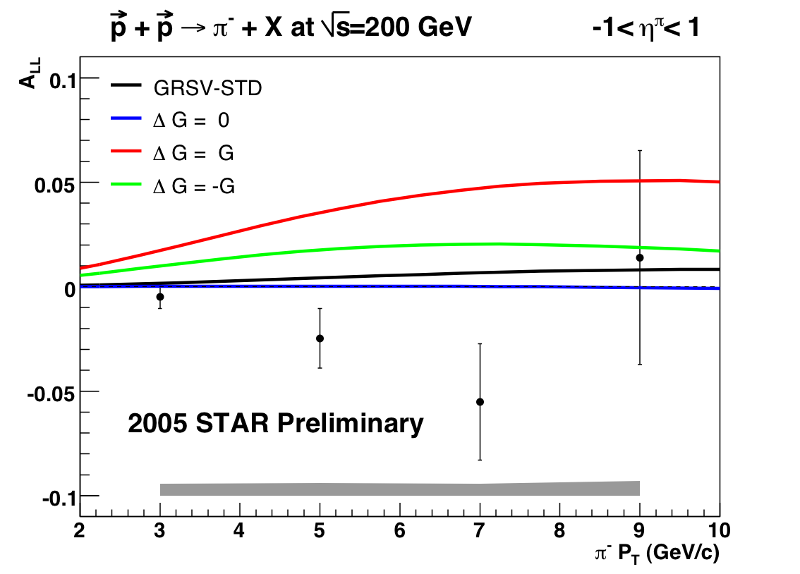
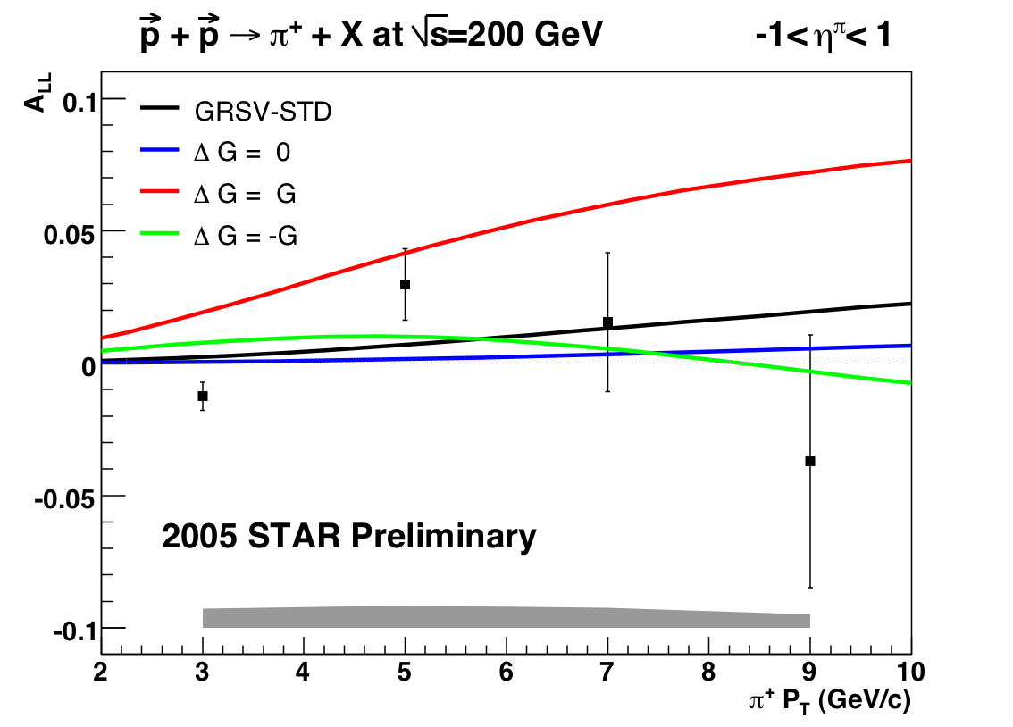
The charged pion A_LL analysis selects pions from events triggered by the EMC. This analysis attempts to estimate the systematic bias introduced by that selection.
Conditions:
- Simulation files, database timestamps, and selection cuts are the same as the ones used in the 2005 Charged Pion Data / Simulation Comparison
- Polarized PDFs are incorporated into simulation via the framework used by the jet group. In particular, only GRSV-std is used as input, since LO versions of the other scenarios were not available at the time.
- Errors on A_LL are calculated according to Jim Sowinski's recipe.
Plots:


Conclusion:
The BBC trigger has a negligible effect on the asymmetries, affirming its use as a "minimum-bias" trigger. The EMC triggers introduce a positive bias of as much as 1.0% in both asymmetries. The positive bias is more consistent in JP2; the HT2 asymmetries are all over the map.
First Look at Single-spin Asymmetries
This is a study of 2005 data conducted in March 2006. Ported to Drupal from MIT Athena in October 2007
eL_asymmetries.pdf
phi_asymmetries.pdf
I also increment 20 separate histograms with (asymmetry/error) for each fill and then fit the resulting distribution with a Gaussian. Ideally the mean of this Gaussian should be centered at zero and the width should be exactly 1. The results are in asymSummaryPlot.pdf
Finally, a summary of single-spin asymmetries integrated over all data. 2-sigma effects are highlighted in bold:
| + | MB | HT1 | HT2 | JP1 | JP2 |
| Y | 0.0691 +/- 0.0775 | 0.0069 +/- 0.0092 | -0.0038 +/- 0.0126 | 0.0086 +/- 0.0104 | 0.0116 +/- 0.0069 |
| B | -0.0809 +/- 0.0777 | -0.0019 +/- 0.0092 | -0.0218 +/- 0.0126 | 0.0067 +/- 0.0104 | -0.0076 +/- 0.0069 |
| - | MB | HT1 | HT2 | JP1 | JP2 |
| Y | -0.0206 +/- 0.0767 | -0.0193 +/- 0.0092 | -0.0158 +/- 0.0130 | -0.0035 +/- 0.0101 | 0.0061 +/- 0.0070 |
| B | 0.0034 +/- 0.0769 | -0.0021 +/- 0.0092 | 0.0006 +/- 0.0130 | -0.0164 +/-0.0101 | -0.0147 +/- 0.0070 |
Conclusions: The jet group sees significant nonzero single-spin asymmetries in Yellow JP2 (2.5 sigma) and Blue JP1 (4 sigma). I do not see these effects in my analysis. I do see a handful of 1 sigma effects and two asymmetries for negatively charged hadrons that just break 2 sigma, but in general these numbers are consistent with zero. I also do not see any significant dependence on track phi.
Inclusive Charged Pion Cross Section - First Look
Correction factors are derived from simulation by taking the ratio of the reconstructed primary tracks matched to MC pions divided by the MC pions. Specifically, the following cuts are applied:Monte Carlo
- |event_vz| < 60.
- |eta| < 1.
- nhits > 25
- geantID == 8||9 (charged pions)
Matched Reco Tracks
- |event_vz|<60.
- |reco eta| < 1.
- |global DCA| < 1.
- reco fit points > 25
- geantID of matched track == 8||9

There is currently a bug in StDetectorDbMaker that makes it difficult to retrieve accurate prescales using only a catalog query for the filelist. This affects the absolute scale of each cross section and data points for HT1 and JP1 relative to the other three triggers. It's probably a 10%-20% effect for HT1 and JP1. With that in mind, here's what I have so far:

This plot is generated from a fraction of the full dataset; I stopped my jobs when I discovered the prescales bug.
The cuts used to select good events from the data are:
- golden run list, version c
- |vz| < 60.
- Right now I am only using the first vertex from each event, but it's easy for me to change
The cuts used to select pion tracks are the same as the ones used for "Matched Reco Tracks", except for the PID cut of course. For PID I require that the dE/dx value of the track is between -1 and 2 sigma away from the mean for pions.
As always, comments are welcome.
Single-Spin Asymmetries by BBC timebin
This is a study of 2005 data conducted in May 2006. Ported to Drupal from MIT Athena in October 2007
Hi jetters. Mike asked me to plot the charged track / pion asymmetries in a little more detail. The structure is the same as before; each column is a trigger, and the four rows are pi+/Yellow, pi+/Blue, pi-/Yellow, pi-/Blue. I've split up the high pt pion sample (2< pT < 12 GeV) and plotted single-spin asymmetries for timebins 7,8, and 9 separately versus pT and phi. The plots and summaries are linked at the bottom of the page.
2 sigma effects are highlighted in yellow, 3 sigma in red. There are no 3 sigma asymmetries in the separate samples, although pi-/B/JP1 is 3 sigma above zero in the combined sample. Here's a table of all effects over 2 sigma:
|
timebin
|
charge
|
trig
|
asym |
effect
|
|
8
|
+
|
HT1
|
Y |
+2.2
|
|
9
|
+
|
JP1
|
B | +2.07 |
| 9 | - | JP1 | B | +2.45 |
| 7-9 | - | JP1 | B | +3.15 |
If you compare these results with the ones I had posted back in March (First Look at Single-spin Asymmetries), you'll notice the asymmetries have moved around a bit for the combined sample. The dominant effect there was the restriction to the new version of Jim's golden run list. The list I had been using before had at least two runs with spotty timebin info for board 5; see e.g.,
http://www.star.bnl.gov/HyperNews-star/protected/get/jetfinding/355/1/1/1.html
and ensuing discussion. I'm in the process of plotting asymmetries for charged track below 2 GeV in 200 MeV pT bins and will post those results here when I have them.
SPIN 2006 Preliminary Result
Event Selection Criteria
- run belongs to golden run list, version c
- BBC timebin belongs to {7,8,9}
- spinDB QA requires: isValid(), isPolDirLong(), !isPolDirTrans(), !isMaskedUsingBX48(x48), offsetBX48minusBX7(x48, x7)==0
- ignore additional vertices
- trigger = MB || JP1 || JP2
- |eta| < 1.
- |global DCA| < 1.
- nFitPoints > 25
- flag > 0
- nSigmaPion is in the range [-1,2]
- Random Patterns
- First Look at Charged Pion Trigger Bias (needs to be updated with more deltaG scenarios, should take ~1 day)
- 2005 Charged Pion Data / Simulation Comparison
- Asymmetries for near-side and away-side pions
- Background from PID Contamination
- Data - Monte Carlo Comparison, Take 2
The following are links to previous studies, some of which are outdated at this point:
Single-Spin Asymmetries by BBC timebin
BBC Vertex
Kasia's estimate of beam background effect on relative luminosities
Kasia's estimate of systematic error due to non-longitudinal porlarization
Asymmetries for near-side and away-side pions
Summary:
I associated charged pions from JP2 events with the jets that were found in these events. If a jet satisfied a set of cuts (including the geometric cut to exclude non-trigger jets), I calculated a deltaR from this jet for each pion in my sample. Then I split up my sample into near-side and away-side pions and calculate an asymmetry for both samples.
Jet cuts:
- R_T < 0.95
- JP2 hardware, software, and geometric triggers satisfied
Note: all plots are pi- on the left and pi+ on the right
This first set of plots shows eta(pion)-eta(jet) on the x axis and phi(pion)-phi(jet) on the y axis. You can see the intense circle around (0,0) from pions inside the jet cone radius as well as the regions around the top and bottom of the plots from the away-side jet:


Next I calculate deltaR = sqrt(deta*deta + dphi*dphi) for both samples. Again you can see the sharp cutoff at deltaR=0.4 from the jetfinder:

 Asymmetries
My original asymmetries for JP2 without requiring a jet in the event:


After requiring a jet in the event I get


Now look at the asymmetry for near-side pions, defined by a cone of deltaR<0.4:


And similarly the asymmetries for away-side pions, defined by deltaR>1.5:


Conclusions: No showstoppers. The statistics for away-side pions are only about a factor of 2 worse than the stats for near-side (I can post the exact numbers later). The asymmetries are basically in agreement with each other, although the first bin for pi+ and the second bin for pi- do show 1 sigma differences between near-side and away-side.
Background from PID Contamination
Summary:The goal of this analysis is to estimate the contribution to A_LL from particles that aren't charged pions but nevertheless make it into my analysis sample. So far I have calculated A_LL using a different dE/dx window that should pick out mostly protons and kaons, and I've estimated the fraction of particles inside my dE/dx window that are not pions by using a multi-Gaussian fit in each pt bin. I've assumed that this fraction is not spin-dependent.
Points to remember:
- my analysis cuts on -1 < nSigmaPion < 2
pi- is on the left, pi+ on the right. Each row is a pt bin corresponding to the binning of my asymmetry measurement. The red Gaussian corresponds to pions, green is protons and kaons, blue is electrons. So far I've let all nine parameters float. I tried fixing the mean and width of the pion Gaussian at 0. and 1., respectively, but that made for a worse overall fit. So far, the fit results for the first two bins seem OK.
2 < pt < 4:
 4 < pt < 6:
 6 < pt < 8:
 8 < pt < 10:

I extracted the the integral of each curve from -1..2 and got the following fractional contributions to the total integral in this band:
| pi- bin | pion | p/K | electron |
| 2-4 | 0.91 | 0.09 | 0.01 |
| 4-6 | 0.92 | 0.05 | 0.03 |
| 6-8 | 0.78 | 0.07 | 0.15 |
| 8-10 | 0.53 | 0.46 | 0.01 |
| pi+ bin | pion | p/K | electron |
| 2-4 | 0.90 | 0.09 | 0.01 |
| 4-6 | 0.91 | 0.06 | 0.03 |
| 6-8 | 0.68 | 0.06 | 0.26 |
| 8-10 | 0.88 | 0.05 | 0.08 |
I repeated my A_LL analysis changing the dE/dx window to [-inf,-1] to select a good sample of protons and kaons. The A_LL I calculate for a combined MB || JP1 || JP2 trigger (ignore the theory curves) is


For comparison, the A_LL result for the pion sample looks like


I know it looks like I must have the p/K plots switched, but I rechecked my work and everything was done correctly. Anyway, since p/K is the dominant background the next step is to use this as the A_LL for the background and use the final contamination estimates from the fits to get a systematic on the pion measurement
Random Patterns
Triggers are| mb | ht1 |
| ht2 | jp1 |
| jp2 | all |
Conclusions: Sigmas of these distributions are ~equal to the statistical error on A_LL. Means are always within 1 sigma of zero
Systematic Error Table
I've included an Excel spreadsheet with currently assigned systematic errors as an attachment.
Run 6
2006 TPC Drift Velocity Investigation
Preliminary analyses of the 2006 data have shown an abnormally large DCA for tracks from a 4-day period following a purge of the TPC on the evening of May 18th. TPC experts have suggested that a recalculation of the drift velocity measurements using the procedure developed for Run 7 may allow for better reconstruction of these tracks. Here's my first attempt at the recalculation, using Yuri's codes "out-of-the-box".Procedure
- Restore st_laser DAQ files from HPSS
- cons StRoot/StLaserAnalysisMaker
- Run a simple BFC chain: root.exe -q -b 'bfc.C(9999,"LanaDV,ITTF","path_to_st_laser_daq_file")'
- execute LoopOverLaserTrees.C+("./st_laser_*.tags.root") to generate drift velocity measurements
Results
Here are the drift velocity measurements currently in the Calibrations_tpc database and the ones that I recalculated from the st_laser DAQ files. I'm only showing measurements from the 10 days around the purge:

I'm not sure how much attention should be paid to the original East laser measurements. The West laser measurements in the DB track pretty closely with the new ones. The significant difference is that there are more new measurements covering the period where the D.V. was changing rapidly:


So what we're really interested in is, for a given event, how different will the D.V. returned by the database be? The way to calculate that is to compare each new measurement to the DB measurement with the closest preceding beginTime:


In the West ratio plot one can clearly see the effect of the additional measurements. For comparison I've plotted the time period where we see problems with the track DCAs and <nTracks> / jet. See for example
http://deltag5.lns.mit.edu/~kocolosk/protected/drupal/4036/summary/bjp1_sum/bjp1_sum_dcaG.gif
http://drupal.star.bnl.gov/protected/spin/trent/jets/2007/apr06/problem_highlights.gif
http://cyclotron.tamu.edu/star/2006Jets/apr23_2007/driftVelocityProb.list
Next Steps
As I mentioned, I didn't tweak any of the parameters on Yuri's codes to get these numbers, so it may be possible to improve them. I looked at the sector-by-sector histograms in the file and the values for the drift velocities looked generally stable. The values for the slopes jumped around a bit more. Assuming there are no additional laser runs that I missed, we could look into interpolating between drift velocity measurements to get even more fine-grained records of the period when the gas mixture was still stabilizing. Here's an example of a fit to the new combined drift velocity measurement in the rapidly-varying region:
References
Discussion on starcalib: http://www.star.bnl.gov/HyperNews-star/get/starcalib/402.htmlEarly Studies
Basic QA Plots
Select a trigger and charge combination to view QA summary plots. Each point on a plot is a mean value of that quantity for the given run, while the error is sqrt(nentries).
Data Collection
Runlist query:
get_file_list.pl -distinct -keys 'orda(runnumber)' -cond 'production=P06ie,trgsetupname=ppProductionLong,sanity=1,tpc=1' -limit 0
This query yields 406 runs (3 with emc=0) which I process with star-submit-template. I'm using Murad's production of StJetSkimEvents to get all event-level info, so my chain is brutally simple: just StMuDSTMaker and a simple set of track quality cuts, viz.
- pT > 2 GeV/c
- |eta| < 2.1
Current working directory (PDSF):
/home/kocolosk/analysis/run6/may03
Once I've got these trees back at MIT I merge them with the jetSkimEvent trees using an index on (run,event) (see Common Analysis Trees). I also apply some more stringent cuts:
Event-level cuts
- spinDB reports all OK
- nVertices > 0 and z-position of best vertex inside 60cm
Track cuts
- pT > 2. GeV/c
- |eta| < 1.
- |DCAglobal| < 1.
- nHitsFit >= 25
- nSigmaPion in [-1,2]
Single Spin Asymmetries by Fill
Away-side only
BJP1 (hardware & software & geometric) requirement, only use pions with dR > 1.5
pi^{+} nSigma asymmetries
fill      yellow     blue       like       unlike
7847      0.7681     0.4152     0.8136     0.2513
7850      0.0743     1.4901     1.1202    -0.9843
7851     -0.5521    -1.5695    -1.5313     0.7059
7852     -0.5546    -1.1228    -1.1148     0.4334
7853     -0.8047     2.7533     1.3496    -2.5720
7855     -0.1095    -1.0144    -0.7683     0.6419
7856      0.6243    -0.6925    -0.0455     0.9280
7858      1.3109     1.9636     2.3779    -0.4507
7863      0.6637     1.3537     1.3883    -0.4979
7864      0.2973    -0.8424    -0.3922     0.7972
7871     -1.7681     0.6963    -0.7669    -1.7202
7872     -1.4830    -0.4183    -1.2917    -0.7713
7883      0.7329    -0.4249     0.2105     0.8539
7886      0.4131     0.7406     0.8332    -0.2265
7887      0.8142     1.0339     1.3192    -0.1441
7896     -0.3938    -0.2628    -0.4542    -0.0927
7901      0.3990     0.0513     0.3428     0.2471
7908     -0.1043    -0.2753    -0.2721     0.1245
7909      0.2401    -1.4131    -0.8252     1.2060
7911     -1.8391     1.9288     0.0727    -2.6732
7913     -0.0822     0.7613     0.4930    -0.5827
7916     -0.3658    -1.9129    -1.5979     1.0991
7918     -1.1823    -0.9377    -1.5543    -0.1821
7921     -0.7642     1.2557     0.3598    -1.4019
7922      1.8057     0.0540     1.2658     1.2471
7926     -0.5481    -2.1827    -1.8897     1.1854
7944      0.0950     0.4734     0.4049    -0.2722
7949     -0.1770     0.6205     0.3156    -0.5489
7951     -0.2755    -0.0891    -0.2622    -0.1306
7952      2.2435     1.6046     2.8193     0.4314
7954     -1.2534    -0.5687    -1.2512    -0.4838
7957     -0.6056    -2.1501    -1.8931     1.1112
pi^{-} nSigma asymmetries
fill      yellow     blue       like       unlike
7847     -0.6434     2.3161     1.1484    -2.1363
7850      1.8693    -0.0728     1.2844     1.3589
7851     -1.2476    -1.4218    -1.9278     0.1198
7852      0.4635    -0.7461    -0.1245     0.9018
7853      0.2474     3.4829     2.6019    -2.3402
7855      0.6099    -0.3582     0.1694     0.7191
7856     -0.3472    -0.0663    -0.3147    -0.2412
7858      0.5772     0.0588     0.4406     0.3577
7863      1.2914     0.4583     1.2065     0.6182
7864      0.9606    -0.4055     0.3951     0.9624
7871     -1.6101    -0.2726    -1.3459    -0.9187
7872      0.5035     0.3827     0.6093     0.0966
7883     -0.7030     0.1324    -0.3950    -0.6150
7886      1.9632     1.2030     2.2793     0.5283
7887      1.1916     1.1695     1.7115     0.0042
7896      1.0944    -1.5376    -0.3071     1.8997
7901     -1.1326    -0.1455    -0.9498    -0.6828
7908     -0.1445     0.6122     0.3287    -0.5444
7909     -1.5394    -0.4124    -1.3598    -0.8080
7911     -2.4637     0.5309    -1.3758    -2.1097
7913      1.4852    -1.7004    -0.1439     2.2214
7916      1.3170    -1.4964    -0.1252     2.0055
7918     -0.0600    -2.4808    -1.8464     1.6679
7921     -0.6402     1.6446     0.6993    -1.5745
7922     -1.7100    -1.8694    -2.4555     0.1048
7926     -0.8854    -1.8649    -1.8962     0.7077
7944      0.7047    -0.3786     0.2404     0.7810
7949     -1.1675     0.2958    -0.6320    -0.9979
7951     -1.6275     0.5100    -0.7990    -1.4975
7952      1.3279     1.7884     2.2557    -0.3194
7954     -0.0209    -0.7787    -0.5861     0.5011
7957      2.2026    -1.9116     0.2045     2.9721
Run 5, inclusive
pi^{-} nSigma asymmetries
fill      yellow     blue       like       unlike
6988      2.8954     3.3548     4.2810    -0.3045
6990     -1.1356     0.0822    -0.7347    -0.8748
6992      2.2104     0.3517     1.9057     1.2493
6994     -0.3457     0.3976     0.0759    -0.6364
6995      0.0236     0.1136     0.1058    -0.0989
6997      0.6616     2.4959     2.2008    -1.2739
6998     -0.0607     0.5594     0.3556    -0.4868
7001     -0.2676     0.5874     0.2397    -0.6092
7002     -1.0157    -1.8627    -2.0789     0.4709
7032     -10.7190     9.6297    -0.9199    -13.3990
7034      2.6986    -1.2420     1.0235     2.7046
7035     -5.9795     5.8657    -0.0851    -8.3401
7048     -0.0177    -1.8298    -1.3617     1.2361
7049     -0.6182    -0.6846    -0.9274     0.0772
7051      1.2298     1.6795     2.1185    -0.3414
7055      0.7022     2.1289     2.0639    -1.0710
7064     -0.4975     1.9746     1.0530    -1.8834
7067     -2.7525     1.7490    -0.6884    -3.2186
7068      0.5999    -2.3405    -1.2244     2.1034
7069      1.6100     1.1541     1.9830     0.3217
7070     -0.0836     0.6656     0.4473    -0.4897
7072      0.1926    -0.7871    -0.3990     0.6684
7075      0.8745    -2.6544    -1.3421     2.4330
7079      0.1552    -1.5263    -1.0723     1.2324
7085     -0.0897    -0.2026    -0.2088     0.0906
7087      1.9237     0.4959     1.6501     1.0719
7088      0.3847    -0.4083    -0.0174     0.5569
7092      2.0581    -0.5933     1.0121     1.9479
7102      0.8406     0.3069     0.7570     0.5024
7103     -0.3106    -1.2057    -1.0763     0.6761
7110      2.6473    -0.2804     1.6718     2.0768
7112      1.5189     0.6019     1.4554     0.7426
7114      1.6817     0.9240     1.7917     0.5391
7118     -1.7624     0.7710    -0.5612    -1.6619
7120     -0.7654     0.2761    -0.2967    -0.7026
7122      0.0848    -0.6810    -0.3646     0.5913
7123     -1.6676     1.3976    -0.0291    -2.0208
7124      1.3759    -0.2691     0.6933     1.2215
7125      1.8810    -0.1630     1.1017     1.5199
7127      0.1055     1.6688     1.1933    -1.1824
7131     -0.1858    -0.0352    -0.2407    -0.1477
7133      0.8733     0.4679     1.0256     0.3223
7134      0.6636    -0.6857    -0.0360     0.9213
7151     -0.3299    -0.6315    -0.7004     0.2166
7153     -2.5741    -1.5110    -3.2579    -0.8339
7161     -0.9482    -0.8973    -1.2234    -0.1557
7162     -1.4261    -0.0548    -1.0450    -0.9047
7164     -0.2787     0.3688     0.1438    -0.5959
7165      0.1723    -1.3462    -0.7982     1.0477
7166      0.3072     2.2635     1.8098    -1.2695
7172     -0.6414     1.0035     0.2382    -1.1475
7237      0.8140    -1.9210    -0.7821     1.9362
7238      0.9147     0.1583     0.7514     0.5303
7249      0.8511     0.0570     0.6455     0.5322
7250      1.6782    -1.6771     0.1037     2.3099
7253      1.2592     0.8287     1.5859     0.2875
7255     -0.1376     0.1269     0.0300    -0.1948
7265     -2.7099    -1.0899    -2.5877    -1.2855
7266     -0.1283     0.7634     0.4338    -0.6211
7269      0.4862    -1.4204    -0.6823     1.3197
7270     -0.3694    -1.4968    -1.3117     0.7702
7271      2.1860     0.7501     2.0633     1.0176
7272      2.2742    -2.2593     0.0511     3.1922
7274      0.3692     1.9398     1.7348    -1.1304
7276     -1.9901     0.5043    -1.0389    -1.7776
7278      0.7444    -0.9791    -0.1687     1.2300
7279     -2.3442     0.9652    -0.9159    -2.3637
7300     -0.8765     1.6118     0.6363    -1.8350
7301      0.8553    -0.2668     0.3570     0.7616
7302      1.0808    -0.0070     0.7584     0.7798
7303     -0.7486     0.1757    -0.3854    -0.6549
7304     -0.7711     0.2501    -0.3825    -0.6815
7305      0.8851     0.7527     1.1938     0.0802
7308     -0.8466     0.7225    -0.0718    -1.1143
7311      0.2896     1.3780     1.1925    -0.7556
7317     -0.8703    -0.0998    -0.6921    -0.5361
7320     -1.3928    -2.0561    -2.4636     0.4663
7325     -0.9948     1.1141     0.0747    -1.5080
7327     -1.6448     0.1399    -1.0593    -1.2770
pi^{-} nSigma asymmetries
fill      yellow     blue       like       unlike
6988      1.5237     0.3259     1.3166     0.8438
6990      1.1388    -0.4585     0.5317     1.0481
6992      2.7809     1.8496     3.2777     0.6367
6994      0.4036    -0.0709     0.2152     0.3816
6995      0.0284     0.7506     0.5669    -0.5518
6997     -1.2708     1.5377     0.1390    -1.9290
6998     -0.2966     0.4639     0.1302    -0.4701
7001      0.8019    -0.9775    -0.1193     1.2528
7002      1.0862    -0.8451     0.1595     1.3065
7032     -7.2733     5.8628    -1.0782    -8.7338
7034      2.4731    -0.8650     1.1370     2.2900
7035     -5.7211     3.9134    -1.2690    -6.7932
7048     -0.9821     0.5199    -0.2484    -0.9325
7049     -2.4413    -1.6901    -2.8984    -0.5287
7051      0.1898     0.2886     0.3473    -0.0752
7055      2.4241     0.6951     2.2625     1.1398
7064      2.2608    -0.4958     1.2645     1.7928
7067     -0.9410    -0.7594    -1.1653    -0.2053
7068      0.2002    -0.1126     0.0601     0.2288
7069      0.6342     0.4304     0.7885     0.1599
7070     -1.2299     2.9297     1.2261    -2.8784
7072     -0.7843     1.6628     0.5990    -1.7002
7075      2.3895    -0.4305     1.3059     1.9201
7079      2.1971    -1.5796     0.3723     2.6978
7085      1.3459    -0.2317     0.7799     1.1367
7087      0.5258     0.2137     0.5551     0.1279
7088     -0.1856    -0.1438    -0.2435    -0.1064
7092      1.2742    -0.2971     0.6764     1.1774
7102     -0.1788     0.7376     0.3437    -0.5362
7103     -0.8089     0.0366    -0.5355    -0.6171
7110      2.6260     0.2961     2.0858     1.6233
7112      1.9199    -0.0349     1.3241     1.3657
7114      1.8546     0.6690     1.6611     0.8189
7118     -1.4017     0.8334    -0.4454    -1.6526
7120     -0.4001    -0.8129    -0.8129     0.3250
7122      0.5141    -0.2102     0.3512     0.6298
7123     -1.3042     1.8959     0.5395    -2.1551
7124      3.9571     0.3816     2.8666     2.6861
7125     -1.3947     0.3251    -0.8597    -1.3188
7127      2.2501    -0.6104     0.9831     2.1725
7131     -0.9200    -0.6472    -1.1191    -0.2102
7133     -1.1714     1.5062     0.0760    -1.9908
7134      0.6319    -1.4622    -0.6012     1.5632
7151      0.5372    -1.7916    -0.9108     1.6296
7153     -1.2329     0.7181    -0.3432    -1.3650
7161      1.3848     0.0689     1.0066     0.8943
7162     -2.3956     0.6038    -1.3699    -2.1493
7164      0.3508     1.6100     1.3783    -0.8174
7165      1.4134    -0.7712     0.4739     1.5248
7166     -0.3523     2.1152     1.2432    -1.6452
7172     -0.1923     3.1633     2.1209    -2.3379
7237      1.5778    -1.1650     0.2675     1.9640
7238      1.4628     3.2685     3.4046    -1.2492
7249      0.4261     0.1171     0.3816     0.2054
7250      1.2336    -1.0578     0.2506     1.5672
7253      0.6686    -1.3123    -0.3461     1.3663
7255      0.4010     0.1360     0.3899     0.1899
7265      0.1921    -1.1813    -0.6969     0.9601
7266     -0.6051    -0.5478    -0.8301    -0.0250
7269      0.1734    -0.5571    -0.2799     0.5063
7270      0.8825    -0.1983     0.4846     0.7612
7271      0.4453    -0.5304    -0.0492     0.6870
7272     -0.0131    -0.0176    -0.1003     0.0666
7274      2.5228    -0.2154     1.7141     1.8915
7276     -1.2212     2.1062     0.6034    -2.3542
7278      0.3318     0.0408     0.2745     0.1836
7279     -0.5121    -1.0690    -1.0773     0.3939
7300     -1.6321     0.7300    -0.6380    -1.6637
7301     -0.3916    -1.4341    -1.3355     0.7032
7302      1.4687    -1.3287     0.0978     1.9877
7303      0.4977     0.8000     0.8904    -0.2186
7304     -1.3292    -1.5037    -2.0497     0.1612
7305      0.2956     1.9077     1.6151    -1.1684
7308     -0.9212    -1.6537    -1.8057     0.5161
7311      0.0845    -1.0962    -0.7150     0.8359
7317     -2.3657    -0.6376    -2.1734    -1.1486
7320     -2.8559     1.1114    -1.2439    -2.7725
7325      0.3738     0.4026     0.5462    -0.0209
7327     -0.0750    -1.3466    -1.0211     0.8721
Preliminary Result
Longitudinal double-spin asymmetries for inclusive charged pion production opposite a jet
Update 2008-10-03: include the effect on A_{LL} from the uncertainty on the jet pT shift in the total point-to-point systematics.

Comparison to models obtained by sampling a_{LL} and parton distribution functions at the kinematics specified by the PYTHIA event:

Asymmetries are plotted versus the ratio of pion p_{T} and the p_{T} of the trigger jet.
Dataset and Cuts
- Runlist (297 long2 runs)
- BJP1 HW+SW trigger (137221, 137222)
- BBC timebin 6-9
- p_{T}(π) > 2.0
- |η_{π}| < 1.0
- |DCA_global| < 1.0
- nHitsFit > 25
- recalibrated nσ(π) in [-1.0, 2.0]
- trigger jet p_{T} in [10.0, 30.0]
- trigger jet detector η in [-0.7, 0.9]
- trigger jet neutral energy fraction < 0.92
- trigger jet ϕ within 36 degrees of fired jet patch center
- Δϕ(trigger jet-pion) > 2.0
Error bars on each histogram take multi-particle correlations into account when multiple pions from an event fall into the same bin. Here is the Δϕ distribution obtained from the data and compared to Monte Carlo:

Systematic Uncertainties
Systematic uncertainties are dominated by the bias in the subprocess mixture introduced by the application of the jetpatch trigger. Uncertainty in the asymmetry of the PID background also contributes in the two highest z bins. The full bin-by-bin systematic uncertainties are
π- = {9.1, 8.1, 6.1, 11.1} E-3
π+ = {14.8, 11.0, 6.6, 14.8} E-3
π- = {9.6, 9.5, 17.1, 14.9} E-3
π+ = {15.3, 13.0, 17.3, 21.8} E-3
Trigger Bias
I initially tried to estimate the bias from the JP trigger by applying the Method of Asymmetry Weights to PYTHIA. The next three plots show the Monte Carlo asymmetries after applying a) the minbias trigger, b) the jetpatch trigger, and c) the difference between a) and b):
a)

b)

c)

As you can see, the bias from this naïve approach is huge. It turns out that a significant source of the asymmetry differences is the fact that each of these bins integrates over a wide range in jet pT, and the mean jet pT in each bin is very different for MB and JP triggers:


We decided to factor out this difference in mean pT by reweighting the minbias Monte Carlo. This reweighting allows the trigger bias systematic to focus on the changes in subprocess mixture introduced by the application of the trigger. Here’s the polynomial used to do the reweighting:

Here are the reweighted minbias asymmetries and the difference between them and the jetpatch asymmetries:


The final bias numbers assigned using GRSV-STD are 6-15 E-3.
PID Background
I calculate the background in my PID window using separate triple-Gaussian fits for π- (8.6%) and π+ (9.2%), but I assume a 10% background in the final systematic to account for errors in this fit:

Then I shift to a sideband [-∞, -2] and calculate an A_{LL}:

The relation between measured A_{LL} and the “true” background-free charged pion A_{LL} is

so the systematic uncertainty we assign is given by

and is ~9 E-3 in the highest bin, 1.5-4 E-3 elsewhere.
Jet pT Shift
I used the corrections to measured jet pT that Dave Staszak determined by comparing PYTHIA and GEANT jets link to correct my measured jet pTs before calculating z. The specific equation is
p_{T,true} = 1.538 + 0.8439*p_{T,meas} - 0.001691*p_{T,meas}**2
There is some uncertainty on the size of these shifts from a variety of sources; I took combined uncertainties from the 2006 preliminary jet result (table at http://cyclotron.tamu.edu/star/2005n06Jets/PRDweb/ currently lists the preliminary uncertainties). The dotted lines plot the 1σ uncertainties on the size of the jet pT shift:

Next I used those 1σ pT shift curves to recalculate A_{LL} versus z. The filled markers use the nominal pT shifts. The open markers to the left plot the case when the size of the shift is large (that is, the 1σ corrected jet pT is lower lower than the nominal case, which causes some migration from nominally higher z into the given bin). The open markers to the right plot the case where the shift is small (corrected jet pT closer to measured).
In short: low markers represent migration from lower z, high markers represent migration from higher z.

No assignment of systematic at the moment. If I were to assign a systematic based on the average difference between the nominal and min/max for each bin I’d get
I assign a systematic based on the average difference between the nominal and low/high for each bin; this ends up being 3-16 E-3.
Relative Luminosity
Murad’s detailed documentation
A pT-independent systematic uncertainty of 9.4 E-4 is assigned.
Non-longitudinal Beam Components
Analysis of beam polarization vectors leads to tan(θB)tan(θY)cos(ΦB-ΦY) = 0.0102. I calculated an Aσ from transverse running:

The small size of the non-longitudinal beam components mean that even the Aσ in the case of π- leads to a negligible systematic on A_{LL}. A pT- and charge-dependent systematic of 1.4-7.3 E-4 is assigned.
Single Spin Asymmetries
The following are summary results (val ± err and χ2) from straight-line fits to single-spin asymmetries versus fill:
| π- | val ± err | χ2 (37 d.o.f.) |
| Y | -4.8 ± 3.0 | 63.74 |
| B | 0.8 ± 3.1 | 34.46 |
| L | 6.7 ± 7.4 | 46.21 |
| U | 9.9 ± 7.5 | 52.51 |
| π+ | val ± err | χ2 (37 d.o.f.) |
| Y | -1.2 ± 2.9 | 53.65 |
| B | 0.5 ± 3.0 | 43.45 |
| L | 3.2 ± 7.2 | 55.03 |
| U | 2.0 ± 7.3 | 41.72 |
There’s a hint of an excess of uu and/or ud counts for π-, but no systematic is assigned.