Modeled distortions

Modeling the Distortion

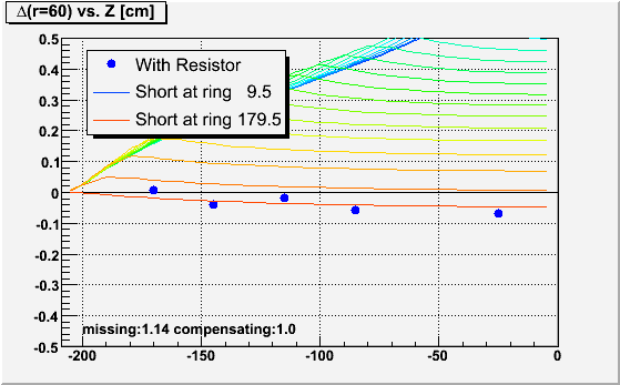
Using StMagUtilities, Jim Thomas and I were able to compare models of the distortions caused by shorts at specific rings in the IFC with the laser data. First, I'll have to say that I was wrong from my Observed laser distortions: the distortion to laser tracks does not have the largest slope at the point where the short is. Instead, it has a maximum at that point! The reason is that the z-component of the electric field due to the distortion (withouth compensating resistor) changes signs at the location of the short. So ExB also changes directions, and the TPC hits are distorted in one rPhi direction on the endcap side of the short, and in the opposite rPhi direction closer to the central membrane.

This can be seen in the following plot, where I again show the distortion to laser tracks at a radius of 60cm (approximately the first TPC padrow) versus Z in the east TPC using distored run 7076029 minus undistorted run 7061100 as red data points. Overlayed are curves for the same measure from models of a half-resistor short (actually, 1.14 MOhm short as determined by the excess current of ~240+/-10nA [a full 2MOhm short equates to 420nA difference]) located at rings 9.5, 10.5, ..., 169.5, 179.5 (there are only 182 rings).

[note: earlier plots I have shown included laser data at Z = -55cm, but I've found that the laser tracks there weren't of sufficient quality to use; I've also tried to mask off places where lasers cross over each other]

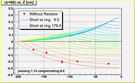
The above plot points towards a short which is located somewhere among rings 165-180 (Z < -190cm). As the previous years' shorted rings were rings 169 and 170 ( = short at ring 169.5), it seems highly likely that the present short is in the same place. More detail can be seen by looking at the actual laser hits. The first listed attached file shows the laser hits as a function of radius for lasers at several locations in Z. The dark blue line is a simple second order polynomial fit I used to obtain the magnitude of the distortion at radius 60cm, which I used in the above plot. The magenta line is the model of the half-resistor short at ring 169.5, and the light blue line is the same for ring 179.5 (the bottom two curves on the above plot). Either curve seems to match the radial dependence fairly well.

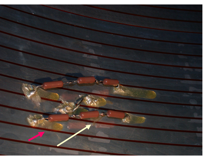
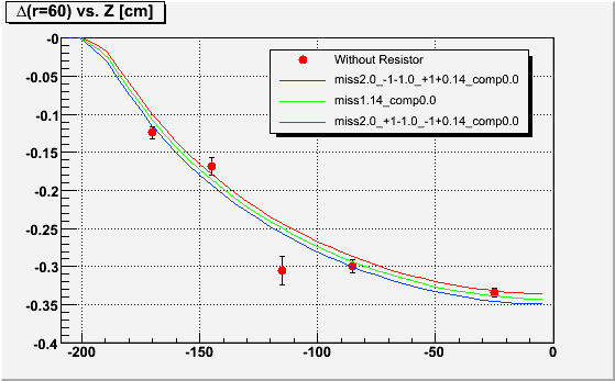
Further refinement can be achieved by modeling the exact resistor chain. We have a permanent short at ring 169.5 (rings 169 and 170 have been tied together), and have replaced the two 2MOhm resistors between 168-169 and 170-171 with two 3MOhm resistors (see the attached photo of the repair, with arrows pointing to candidate locations for shorts via drops of silver epoxy). So it is more likely that we have a 1.14MOhm short on one of these two 3 MOhm resistors. The three curves in this next plot are:

red: 1.14MOhm short on a 3MOhm resistor at 168.5, full short at 169.5, 3MOhm resistor at 170.5
green: 1.14MOhm short on a 2MOhm resistor at 169.5, normal 2.0MOhm resistors at 168.5 and 170.5
blue: 3MOhm resistor at 168.5, full short at 169.5, 1.14MOhm short on a3MOhm resistor at 170.5

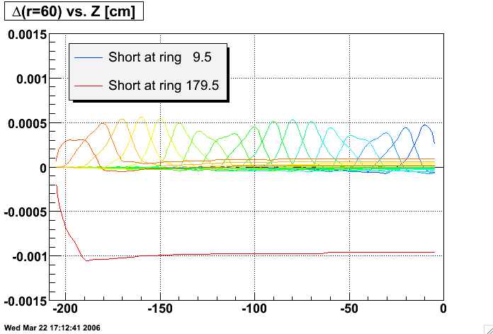
The difference between the curves does not come from the fact that we have treated the 3MOhm resistors properly (that difference is less than 5 microns in distortions, and only in a small region near the short! shown here), but rather from the movement of the effective short from location 168.5 to 169.5 to 170.5. From a visual inspection (not a fit), it appears that the blue curve is the best match to the data:

We can also take a look at the data with the resistor in. Here is the same plot as before with a 1.14MOhm short at the same locations, but with an additional compensating resistor of 1.0MOhm. The fact that all the data points are below zero points again towards a short near the very end of the resistor chain, preferring a location of perhaps 177.5 over shorts near ring 170. These plots do not include the use of the 3MOhm resistors, but that difference is below the resolution presented here.

Zoom in with finer granularity between rings (every other ring short shown):

The second listed attached file shows the laser hits as a function of radius for lasers at several locations in Z for the case of the resistor in, again with magenta and blue curves for the model with shorts at ring 169.5 and 179.5 respectively.

Applying the Correction

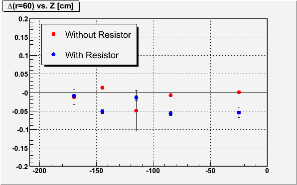
I tried running reconstruction on the lasers using the distortion corrections for the 1.14MOhm short at three locations: 170.5 and 171.5 (two possible spots indicated in Alexei's repair photo), and 175.5 (closer to what the with-resistor data pointed to). The results are in the following plots. The conclusion is that the 175.5 location seems to do pretty well at correcting the data, slightly better than the 170.5 and 171.5 locations, for both with and without compensating resistor. For this reason (the laser data), we will proceed with FastOffline using a short at 175.5, even though we have no strong reasons outside the laser data to suspect that the short is anywhere other than the rings 168-172 area where the fix was made.

170.5	171.5	175.5

Gene Van Buren
gene@bnl.gov

Choosing an external resistance for an IFC short

It is clear that when a field cage short is close to the endcap, it is best to add an external resistance to compensate for the amount of the missing resistance from the short as that would restore the current along the length of the resistor chain and only disrupt the potential at the last (outermost) rings instead of along the full length. A short near the central membrane would benefit less from this as restoring the proper current does restore the potential drop between each ring, but leaves almost all rings at a potential offset from the intended potential, essentially tilting the E field over nearly the whole volume.

But the question then comes as to whether we can decide on the best external resistance for minimizing the distortion, to align with the principle that the best distortion we can choose is the one which requires the least correction, in case we're not quite correcting it accurately. To answer that, the distortion modeling was run with a variety of locations for an IFC west 2 MOhm single-resistor short, and a variety of external resistances. The code to run this modeling has been attached as a tar file to this Drupal page in case there is interest to re-run it (e.g. for an OFC short).

Here are the results:

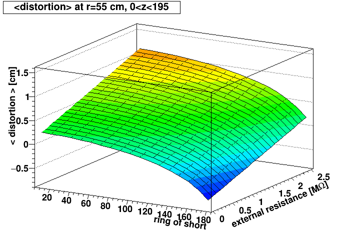
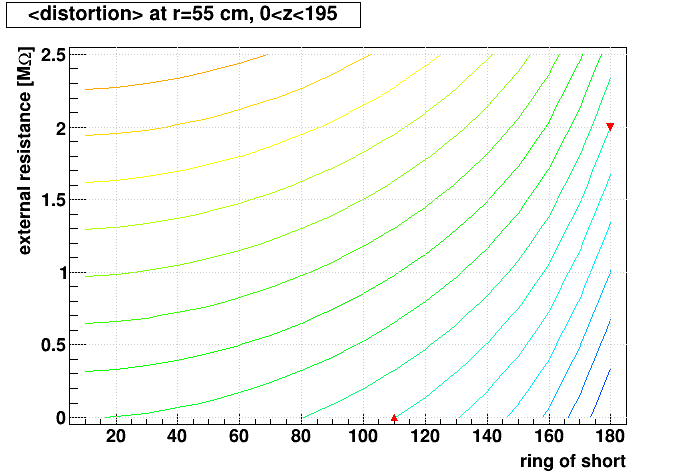
Left: Surface plot showing the mean r-φ distortion we would get at the first iTPC pad row (radius = 55 cm) averaged over all active west-side z as a function of where the short is located ("ring of short") and how much external resistance is added.
Right: Same but drawn as contours. The curve of interest to follow, that leads to <distortion>=0, is the one that starts near (ring,external resistance) = (110,0.0) and ends near (180,2.0), as indicated by the red markers. If the short is at ring 160.5, for example, then this curve indicates an external resistance of ~1.05 MΩ minimizes the distortions averaged over all active west-side z.

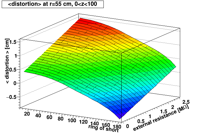
However, it may be more important to restrict the z range included in the distortion average, as most tracks of interest do not cross the inner pad rows at high z...

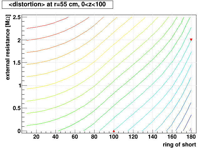
Left: Similar surface plot, but restricting the average to 0 < z < 100 cm.
Right: The curve of interest to follow in this contour plot, that leads to <distortion>=0, is the one that starts near (100,0.0) and ends near (180,2.0), as indicated by the red markers. If the short is at ring 160.5, then this curve indicates that an external resistance of ~1.25 MΩ minimizes the distortions averaged over 0 < z <100 cm.

Some additional observations:

The curve of interest should always end close to (180.5,2.0), as that approaches the condition where the external resistance is no different than an internal resistance at the very end of the chain.
The above is a simplification of what area should be integrated, as tracks with η ≠ 0 cross a variety of z at various radii, complicating the impact on their reconstruction. A track-by-track analysis of impact would be more meaningful, but a lot more work! The modeling shown here can serve as a rough guide to the best external resistance to use, but should not be taken as definitive for all physics.
It is interesting to note that the model implies that a negative external resistance would help minimize the <distortion> when the short is closer to the central membrane (ring 0). A way to think of this is like having a short at both ends, such that the potentials are too high near the central membrane, and then too low near the endcap, so that the E field tilts one way in the region near the central membrane, isn't tilted at half the drift length, and then tilts the other way near the endcap, resulting in opposing distortions for electrons which drift the full length that serve to cancel each other. This could in principle be achieved by reducing the overall resistance of the Resistor box at the end of the Field Cage chain. The STAR TPC has (as of this documentation) had no persistent shorts near the central membrane that would warrant this approach.

-Gene

OFC West possible distortion

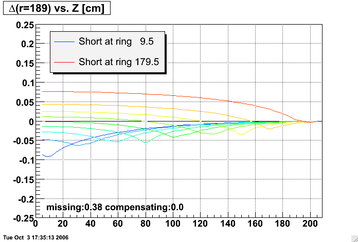
There remains a possible distortion due to a potential short in the OFC west as well. We see a bimodal pattern of 0 or 80 excess nanoAmps coming out of the OFC West field cage resistor chain (it has been there since the start of the 2005 run). That corresponds to a 0.38 MOhm short (420nA = 2 MOhms). The corresponding distortion depends on the location of the electrical short. The plot shown here is the distortion in azimuth (or rPhi) at the outermost TPC padrow near the sector boundaries (r=195 cm, the pads are closer to the OFC near the sector boundaries) due to such a short between different possible field cage rings:

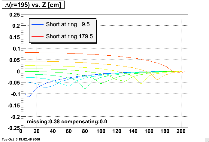
In terms of momentum distortion, a 1mm distortion at the outermost padrows would cause a sagitta bias of perhaps about 0.5mm for global tracks (and even less for primary tracks), corresponding to an error in pt in full field data of approximately 0.006 * pt [GeV/c] (or 0.6% per GeV/c of pt). This is certainly at the level where it is worthwhile to try to fix the distortion if we can figure out where the short is. It is also at the level where we should be able to see with the lasers perhaps to within 50cm where the short is.

Just as a further point of reference, the plot for radius = 189cm, corresponding to the radius of the outermost padrow in the middle of a sector (its furthest point from the OFC) can be found here.

This possible distortion remains uninvestigated at this time.

Gene Van Buren
gene@bnl.gov

Other FC short distortion measurements

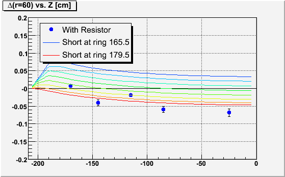
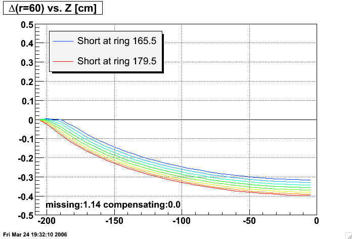
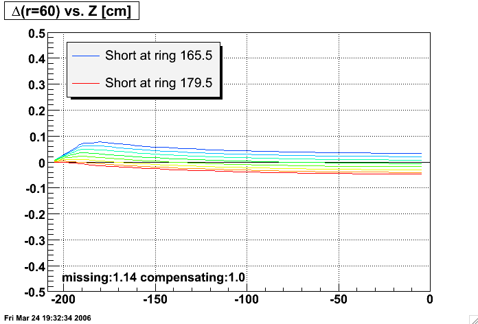
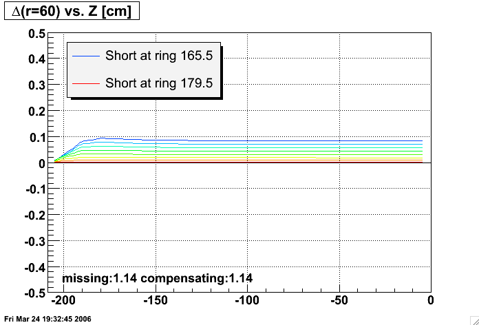
I considered the possibility that other measurements might help isolate the location of the short in the TPC. So, using the Modeled distortions, I modeled the effects of adding even more compensating resistance to the end of the IFC east resistor chain. Below are the results for shorts located at ring 165.5 (between rings 165 and 166), 167.5, 169.5, ..., 179.5 as indicated for the colored curves. All plots use a 1.0cm range on the vertical scale so that they can be easily compared. I had hoped that one resistance choice or another would cause more separation between the curves, giving better resolving power between different short locations. But this dependence is small, and actually seems to decrease a little with increased compensating resistance. Remember also that the last laser is at Z of about -173cm.

Also perhaps worth noting is that the 1.0MOhm compensating resistor probably helps reduce the distortions even more than an exact 1.14MOhm would. The latter causes the distortions not to change between the short location and the central membrane, but the former actually causes the distortion to re-correct the damage done between the short location and the endcap!

Compensating resistance [MOhms]	Distortion on first padrow vs. Z
0.0
1.0
1.14
2.0
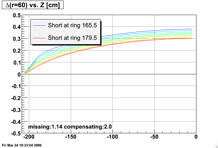4.0
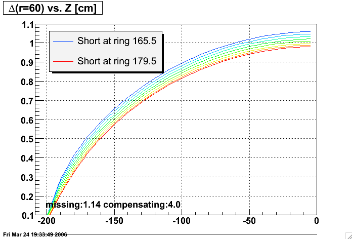20.0

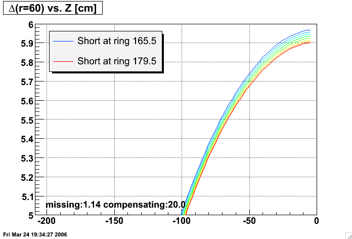Gene Van Buren
gene@bnl.gov