Run 6 Neutral Pions
Neutral pion analysis
2006 Neutral Pion Paper Page
Proposed Title: "Double longitudinal spin asyymetry and cross sectrion for inclusive neutral pion production at midrapidity in polarized proton collisions at Sqrt(s) = 200GeV"
PAs: Alan Hoffman, Joe Seele, Bernd Surrow, ...
Target Journal: PRD - Rapid Communication
Abstract:
Figures:
The first two figures are obvious: the cross section plot and the A_LL plot. The third is less so. I offer a number of options below.
1)
Caption 1. Cross section for inclusive \pi^0 production. a) The unpolarized cross section vs. P_T. The cross section points are plotted along with NLO pQCD predictions made using DSS and KKP fragmentation functions. b) Statistical and systematic uncertainties for the cross section measurement. c) Comparison of measured values to theoretical predictions. Predictionsa re shown for three different fragmetnation scales to give an idea of theoretical uncertainty.
2)
Caption 2. The longitudinal double spin asymmetry, A_LL, vs. P_T for inclusive \pi^0 prodution. The error bars are purely statistical. The systmatic uncertainty is represented by the shaded band beneath the points. The measurement is compared to a number of NLO pQCD predictions for different input values of \Delta G.
3) Option 1
Caption: Comparison between Data and Simulation for energy asymmetry Z_gg = |E1 - E2|/(E1 + E2). (Ed. Note: The nice thing about this plot is that it would not require too much supporting explanation in the text. Readers would know what it means. "Monte Carlo" could be changed to "Pythia + Geant" to be more specific.)
3) Option 2
Caption: Left: Two photon invariant mass distribution for data (black points) and various simulation components. Right: Same data distribution compared to combined simulation. (Ed. Note: This plot would require us to describe the whole mass-peak simulation scheme, which may be outside the scope of the paper.)
3) Option 3
Some combination of these two plots showing the A_LL points and then the P-values associated with various pQCD predictions. This would follow the example set by the jet group.
Summary and Conclusions:
Supporting Documentation:
2006 Neutral Pion Update (9/27/07)
Click on the link to download my slides for the PWG meeting.
A_LL
BEMC Related Studies
My initial attempt at pinpointing the causes of the 'floating' pion mass examined, as possible causes, the fit function, an artificial increase in the opening angle, and the BEMC energy resolution. Preliminary findings indicate that the both the opening angle and the BEMC resolution play a part in the phenomena, however the resolution seems to be the dominant factor in these pt ranges (5.2 - 16).
I also compared the effect in Data and MC using a full QCD (pythia + geant) MC sample, filtered for high-pt pions. As can be seen in the link below, the mean mass position and peak widths are comprable in data and MC. The floating mass problem is readily reproduced in this MC sample.
Cross Section Analysis
On the pages listed below I'm going to try to keep track of the work towards measuring the cross section for inclusive pion production in pp collisions from run 6. I'll try to keep the posts in chronological order, so posts near the bottom are more recent than posts near the top.
- Data Sets
- Candidate Level Comparisons
- Special attention to Zgg
- Data/Full Pythia Inv. Mass comparison (1st try)
- 'Jigsaw' Inv Mass Plot (1st try)
- 'Jigsaw' Inv Mass Plot (2nd try)
- 'Jigsaw' Inv Mass Plot (final)
- Correction Factor (Efficiency)
- Concerning the 'floating' mass peak and Zgg
- Fully Corrected Yields
- Systematic Uncertainties from Background Subtraction and Correction Factor (The Baysian Way)
- Systematic Uncertainty from BEMC energy scale
- Systematic from Cut variations
- Total Errors and Plot
- Preliminary Plot
- Preliminary Presentation
- Comparison with Other Results
- Mass peak Data/MC comparison
- Concerning the High-Mass Tail on the Pion Peak
All Errors
The plot below shows the total errors, statistical and systematic, for the cross section measurement. The inner tick marks on the error bars represent the statistical errors. The outer ticks represent the statistical and point-to-point systematic errors added in quadrature. The grey band shows the systematic error from the BEMC gain calibration uncertainty, which we have agreed to separate from the others (as it cannot be meaningfully added in quadrature to the other uncertainties).
BEMC Calibration Uncertainty
Goal:
To calculate the systematic uncertainty on the cross section due to the BEMC calibration uncertainty.
Justification:
Clearly, the BEMC energy scale is of vital importance to this measurement. The energies measured by the BEMC are used to calculate many of physics level quantities (photon energy, pion pt, pion mass, Zgg) that directly enter into the determination of the cross section. Since the calibration of the BEMC is not (and indeed could not be) perfect, some level of uncertainty will be propagated to the cross section. This page will try to explain how this uncertainty is calculated and the results of those calculations.
Method:
Recently, the MIT grad students (lead by Matt Walker) calculated the gain calibration uncertainty for the BEMC towers. The results of this study can be found in this paper. For run 6, it was determined that the BEMC gain calibration uncertainty was 1.6% (in the interest of a conservative preliminary estimate I have gone with 2%). In the analysis chain, the BEMC gains are applied early, in the stage where pion candidate trees are built from the MuDSTs. So if we are to measure the effect of a gain shift, we must do so at this level. To calculate the systematic uncertainty, I recalculated the cross section from the MuDSTs with the BEMC gain tables shifted by plus or minus 2%. I recreated every step of the analysis from creating pion trees to recreating MC samples, calculating raw yields and correction factors, all with shifted gain tables. Then, I took the ratio of new cross section to old cross section for both shifts. I fit these ratios after the first two bins, which are not indicative of the overall uncertainty. I used these fits to estimate the systematic for all bins. The final results of these calculation can be found below.
Plots:
1) All three cross secton plots on the same graph (black = nominal, red = -2%, blue = +2%)
2) The relative error for the plus and minus 2% scenarios.
Discussion:
This method of estimating the systematic has its drawbacks, chief among which is its maximum-extent nature. The error calculated by taking the "worst case scenario," which we are doing here, yields a worst case scenario systematic. This is in contrast to other systmatics (see here) which are true one-sigma errors of a gaussian error distribution. Gaussian errors can be added in quadrature to give a combined error (in theory, the stastical error and any gaussian systematics can be combined in this manner as wel.) Maximum extent errors cannont be combinded in quadrature with gaussian one-sigma errors (despite the tendency of previous analyzers to do exactly this.) Thus we are left with separate sources of systematics as shown below. Furthermore, clearly this method accurately estimates the uncertainty for low pt points. Consider, for example, the +2% gain shift. This shift increases the reconstructed energies of the towers, and ought to increase the number of pion candidates in the lower bins. However, trigger thresholds are based on the nominal energy values not the increased energy values. Since we cannot 'go back in time' and include events that would have fired the trigger had the gains been shifted 2% high, the data will be missing some fraction of events that it should include. I'm not explaining myself very well here. Let me say it this way: we can correct for thing like acceptence and trigger efficiency because we are missing events and pions that we know (from simulation) that we are missing. However, we cannot correct for events and candidates that we don't know we're missing. Events that would have fired a gain shifted trigger, but didn't fire the nominal trigger are of the second type. We only have one data set, we can't correct for the number of events we didn't know we missed.
All this being said, this is the best way we have currently for estimating the BEMC energy scale uncertainty using the available computing resources, and it is the method I will use for this result.
Candidate Level Comparisons
Objective:
Show that, for an important set of kinematic variable distributions, the full QCD 2->2 Pythia MC sample matches the data. This justifies using this MC sample to calculate 'true' distributions and hence correction factors. All plots below contain information from all candidates, that is, all diphoton pairs that pass the cuts below.
Details:
Data (always black points) Vs. T2_platinum MC (always red) (see here)
Cuts:
- Events pass L2gamma software trigger and (for data) online trigger.
- candidate pt > 5.5
- charged track veto
- at least one good strip in each smd plane
- Z vertex found
- | Z vertex | < 60 cm
Plots:
1a)
The above plot shows the Zgg distribution ((E1 - E2)/(E1 + E2)) for data (black) and (MC). The MC is normalized to the data (total integral.) Despite what the title says this plot is not vs. pt, it is integrated over all values of pt.
1b)
The above left shows Data/MC for Zgg between 0 and 1. The results have been fit to a flat line and the results of that fit are seen in the box above. The above right shows the histogram projection of the Data/MC and that has been fit to a guasian; the results of that fit are shown.
2a)
The above plot shows the particle eta for data pions (black) and MC pions (red). The MC is normalized to the data (total integral.) As you can see, there is a small discrepancy between the two histograms at negative values of particle eta. This could be a symptom of only using one status table for the MC while the data uses a number of status tables in towers and SMD.
2b)
The above left plot shows Data/MC for particle eta, which is fit to a flat line. The Y axis on this plot has been truncated at 2.5 to show the relevant region (-1,1). the outer limits of this plot have points with values greater than 4. The above right shows a profile histogram of the left plot fit to a gaussian. Note again that some entries are lost to the far right on this plot.
3)
The above plot shows detector eta for data (black) and MC (red). Again we see a slight discrepancy at negative values of eta.
3b)
The above left shows Data/MC for detector eta, and this has been fit to a flat line. Again note that the Y axis has been truncated to show detail in the relevant range. The above right shows a profile histogram of the left plot and has been fit to a guassian.
4)
The above plot shows the raw yields (not background subtracted) for data (black) and MC (red) where raw yield is the number of inclusive counts passing all cuts with .08 < inv mass < .25 and Zgg < 0.7. There is a clear 'turn on' curve near the trigger threshold, and the MC follows the data very nicely. For more information about the individual mass peaks see here.
Conclusions:
The Monte Carlo sample clearly recreates the data in the above distributions. There are slight discrepancies in the eta distributions, but they shouldn't preclude using this sample to calculate correction factors for the cross section measurement.
Collaboration Meeting Presentation and wrap up.
Attached is the presentation I gave at the collaboration meeting in late March. It was decided that before releasing a preliminary result, we would have to calculate the BEMC gain calibration uncertainty for 2006. A group of us at MIT created a plan for estimating this uncertainty (see here) and are currently working on implementing this plan as can be seen in Adam's blog post here:
http://drupal.star.bnl.gov/STAR/blog-entry/kocolosk/2009/apr/06/calib-uncertainty-update.
We hope to have a final estimate of this uncertainty by early next week. In that case, I can hopefully calculate the uncertainty in the cross section by the spin pwg meeting on 4/23. If this can be done, I will present the results then and ask to release the preliminary result for DIS 2009. If we cannot calculate a gain calibration systematic by 4/23, obviously we will not be asking to release the preliminary result.
Comparison with Other Results
Below you will find comparisons of the Run 6 cross section with recent Phenix results and the STAR Run 5 final result. The lower panel is the statistical error on the Run 6 points. Uncertainties for the other plots are not included. Plot 1 shows a comparison between run 6 and the Phenix result as published in PRD. Plot 2 shows a comparison between run 6 and the Run 5 final result from STAR, and plot three 3 shows all three results together. As requested, I included the errors for both run 5 and 6 results. The error bars on the cross section points are a quadrature sum of all errors (stat and sys) for the results.
Concerning the 'floating' mass peak and Zgg
Objective:
Explore the pt-dependent mean mass position in data and MC and perhaps draw some conclusions about the quality of our simulations.
Details:
Data Vs T2 platinum MC (see here for explanations)
Bins in Pt {5.5, 6., 6.75, 7.5, 8.25, 9.25, 11., 13., 16., 21.}
Cuts:
- Events pass L2gamma software trigger and (for data) online trigger.
- candidate pt > 5.5
- charged track veto
- at least one good strip in each smd plane
- Z vertex found
- | Z vertex | < 60 cm
Plots:
1)
The above plot shows data (black) Vs. MC (red) for Zgg for my 9 pt bins. The MC plots are normalized to the data so that the total number of entries is equal in both distributions.
2)
Apologies for the poor labeling. The above left plot shows the mean mass per Pt for data (black) and MC (red). These means are calculated by fitting the mass spectra to a gaussian between .1 and .2 GeV/c^2. (see here for more) In addition to the cuts listed at the top of page, I make a Zgg < .7 cut and an | particle eta | < .7 cut on all pion candidates. The PDG mass of the pi0 is shown in blue. The above right plot shows the ratio of Data/MC for the mean masses, again as a function of Pt. This plot is fit to a flat line and the fit parameters are shown.
Conclusions:
The most basic conclusion we can draw is that the simulation is recreating the floating mass peak quite well. The data is never more than 3% higher or lower than the simulation and a flat-line fit is really darn close to one. Couple this with the Zgg comparison and I think we can say that we are simulating the EMC (and SMD) response correctly, at least as it concerns reconstructing neural pions between 5 - 20 GeV/c. Of particular interest is the Zgg comparisons at relatively higher Pt, as then the distance between the two reconstructed photons is smaller than the size of one tower, and we rely on the SMD to correctly identify the daughter photons.
Concerning the High Mass Tail on the Pion Peak
At the PWG meeting a few weeks ago, people expressed concerns about the high-mass tail from the pion peak that, for higher PT bins, is underestimated by the pion peak simulation. This is shown (in the most egregious case) below (see especially, the left-hand plot between .2 and .5):
It is clear, at least at high-pt that the aggregate MC model does not fully reproduce this 'bleeding edge'. Naturally the question arises of how sensitive the cross section measurement is to this tail. One way to probe the sensitivity is to vary the invariant mass cut around the peak position. For the preliminary result, I used a 3 sigma cut calculated by fitting the mass peak to a gaussian. I can also calculate the cross section using a 2 sigma and 4 sigma cut. These cuts are shown below...
This plot shows a closeup of the pion peak for each of the 9 bins, with vertical lines showing the three different mass windows. For most bins, the 2 sigma cut completely excludes the tails and the 4 sigma cut includes a large portion of the tails.
I can then compare the different windows to the nominal window and the smaller (larger) windows.
| Bin | % diff 4 sig | % diff 2 sig |
| 1 | 2.4 | 1.4 |
| 2 | 1.6 | 0.5 |
| 3 | 3.3 | 1.7 |
| 4 | 6.2 | 3.0 |
| 5 | 5.6 | 4.5 |
| 6 | 10.6 | 4.8 |
| 7 | 10.3 | 5.3 |
| 8 | 13.5 | 2.3 |
| 9 | 10.1 | 0.62 |
The largest % difference is 13.5%, in the 8th bin. For the most part the higher pt bins can be off by ~10% for a large mass window.
Cut Variation Tests
Goal:
To test the stability of the cross section measurement to changes in the analysis cuts and, if necessary, assign a systematic uncertainty for cut variations.
Justification:
At many points in the measurements I make cuts on the data. For example, I place a maximum Zgg cut of 0.7 on all pion candidates. These cuts are motivated by our understanding of the detector and underlying physics, but the specific location of each cut is somewhat arbitrary. The cuts could move by some small amount and still be well-motivated. The measurement should be relatively stable with respect to changing analysis cuts. To test this, I take the three most important cuts, Zgg, inv. mass window, and z vertex, and vary them by some small amount in either direction. I then repeat the analysis from start to finish to discern the effect (if any) these cut changes have on the final cross section. The procedure is similar to that used to test the BEMC energy scale systematic (seen here)
Plots:
Instead of showing the cross section measurement for each individual cut change, I will plot the results in what I hope is a more illuminating way. Below is nine plots, each one representing a Pt bin in my analysis. The Pt range in GeV/c is shown in the upper right hand corner. Plotted on each canvas are the (Delta Sigma)/(Sigma) points for each of the cut variations (see key below.) Also note the solid lines indicating the statistical error of the nominal cross section measurement in that bin.
KEY:
point x position Cut Change
2 Invariant Mass Window of plus/minus 4sigma (nominal is 3sigma)
3 Zgg - 10%
4 Z vertex cut + 10%
7 Invariant Mass Window of plus/minus 2sigma (nominal is 3sigma)
8 Zgg cut - 10%
9 Z vertex - 10%
Broadly speaking, the points on the left side of the dashed-dotted line at 5.5 are cut changes that ought to increase raw yield and cuts on the right side ought to decrease raw yield. Of course an increase (decrease) in raw yield does not always translate into an increase (decrease) in cross section because the raw yields are corrected. Note that for most bins the effect for all cut changes is small (on the same order as the statistical uncertainty.) Other systematics (BEMC energy scale and yield extraction) dominate the uncertainty.
Data MC comparison
Data and MC comparison for pion mass peak position..
The left side shows the individual mass peak positions for Data (black) and MC (red). The MC points trend a touch higher than the data point. On the right is (Data-MC)/MC. The right side plot is fit to a pol0, the value of the fit is shown to be -1.01%.
Data Sets
For the cross section analysis I am using a number of Monte Carlo samples along with one data set. The details of each of these sets can be found below:
Pion enhanced, QCD 2->2 sample (full event): aka "T2 Platinum":
This MC sample was produced at Tier 2 by Mike Betancourt for me. It consists of ~200,000 events in each of following partonic pt bins {5-7, 7-9, 9-11, 11-15, 15-25, 25-35} GeV. The events were pre-filtered at the pythia level so every event contains a pythia-level pion with the following kinematic cuts: Pt > 4 GeV, -1.2 < particle eta < 1.2. The code to generate the trees lives on /star/u/ahoffman/T2_maker and is complied in SL08c. The MuDsts and .geant files are archived at HPSS. The trees themselves (600 files) live on /star/institutions/mit/ahoffman/Pi0Analysis/T2_platinum/Trees/. The following parameters were set in the analysis macro:
- db1->SetDateTime(20060522,93000);
- //variables for the trig simulator
int flagMC=1; // 0== off
int useEemc=1; // 0== off
int useBemc=1; // 0== off
int useL2=1; // 0== off
int L2ConfigYear = 2006; //possible 2008
int bemcConfig=2; // enum: kOnline=1, kOffline, kExpert
int playConfig=100; // jan:100_199
int emcEveDump=0; // extrating raw EMC data in a custom format
char *eemcSetupPath="/afs/rhic.bnl.gov/star/users/kocolosk/public/StarTrigSimuSetup/"; - //Settings for Emc simu maker:
int controlval = 2;emcSim->setCalibSpread(kBarrelEmcTowerId,0.15);
emcSim->setCalibOffset(kBarrelEmcTowerId,0.);
emcSim->setCalibSpread(kBarrelSmdEtaStripId,0.25);
emcSim->setCalibOffset(kBarrelSmdEtaStripId,0.0);
emcSim->setMaximumAdc(kBarrelSmdEtaStripId,700);
emcSim->setMaximumAdcSpread(kBarrelSmdEtaStripId,70);
emcSim->setCalibSpread(kBarrelSmdPhiStripId,0.25);
emcSim->setCalibOffset(kBarrelSmdPhiStripId,0.0);
emcSim->setMaximumAdc(kBarrelSmdPhiStripId,700);
emcSim->setMaximumAdcSpread(kBarrelSmdPhiStripId,70); - pre_ecl->SetClusterConditions("bemc", 4, .4, .05, 0.02, kFALSE);
pre_ecl->SetClusterConditions("bsmde", 5, 0.4,0.005, 0.1,kFALSE);
pre_ecl->SetClusterConditions("bsmdp", 5, 0.4,0.005, 0.1,kFALSE);
As of now, only events which pass the software trigger conditions for trigger 137611 (HTTP L2gamma) or 117001 (mb) are saved. These events are weighted properly using Mike B's custom weight calculator for his filtered events. That code can be found /star/u/ahoffman/BetanWeightCalc/
Single Particle Monte Carlo Sets
I have three separate single particle MC samples, single pion, single eta, and single gamma. These were produced using the code located at /star/u/ahoffman/SingleParticle_platinum/. The starsim, bfc, and treemaking code is all there. The .MuDsts and .geant files that result from the bfc jobs are run through a treemaker similar to that for the full pythia monte carlo. These samples are used to estimate the background shapes in in the diphoton invariant mass spectrum. The single gamma sample, for example, is used to model the 'low mass' background, as pion candidates are found from split clusters. The following cuts were set in the macro:
- db1->SetDateTime(20060522,93000);
- //settings for emc simu maker:
int controlval = 2;emcSim->setCalibSpread(kBarrelEmcTowerId,0.15);
emcSim->setCalibOffset(kBarrelEmcTowerId,0.);
emcSim->setCalibSpread(kBarrelSmdEtaStripId,0.25);
emcSim->setCalibOffset(kBarrelSmdEtaStripId,0.0);
emcSim->setMaximumAdc(kBarrelSmdEtaStripId,700);
emcSim->setMaximumAdcSpread(kBarrelSmdEtaStripId,70);
emcSim->setCalibSpread(kBarrelSmdPhiStripId,0.25);
emcSim->setCalibOffset(kBarrelSmdPhiStripId,0.0);
emcSim->setMaximumAdc(kBarrelSmdPhiStripId,700);
emcSim->setMaximumAdcSpread(kBarrelSmdPhiStripId,70);
- pre_ecl->SetClusterConditions("bemc", 4, .4, .05, 0.02, kFALSE);
pre_ecl->SetClusterConditions("bsmde", 5, 0.4,0.005, 0.1,kFALSE);
pre_ecl->SetClusterConditions("bsmdp", 5, 0.4,0.005, 0.1,kFALSE);
pre_ecl->SetClusterConditions("bprs", 1, 500., 500., 501., kFALSE);
One important difference to note is that these events are not held to the simulated trigger standard. Instead, I only choose events (offline) that have pion candidates with Pt above the trigger threshold. Essentially this assumes that the trigger efficiency is perfect for such events. Obviously this is not true, but in my analysis these samples are used primarily to estimate the background line shapes. The single pion events are not weighted. The other two samples are weighted according to the funcional form given by the PHENIX cross section measurements.
Data
This analysis is only concerned with run 6 data, and only data that satisfies the HTTP L2gamma trigger (online and software.) I restrict myself to good runs between 7139017 and 7143025, as it is the longest period of run 6 with relatively stable tower and SMD status tables. Parts of the barrell are missing in this run range, and this will be accounted for in a geometric acceptance correction, but I believe that the stability of the status tables is more important that having a 100% live detector. Using a stable run range will cut down on the systematic error of the measurement which, given previous measurements, will be larger than the statistical error. The data was produced by Murad using my StSkimPionMaker (which can be found in StSpinPool) as part of the SpinAnalysisChain. The output trees are located at /star/institutions/mit/ahoffman/Pi0Analysis/Murads_Production_2_08/. The following parameters were made in the macro:
-
//Get TriggerMaker
StTriggerSimuMaker *simuTrig = new StTriggerSimuMaker("StarTrigSimu");
simuTrig->setMC(false); // must be before individual detectors, to be passed
simuTrig->useBbc();
simuTrig->useBemc();
simuTrig->bemc->setConfig(StBemcTriggerSimu::kOffline);
StGenericL2Emulator* simL2Mk = new StL2_2006EmulatorMaker;
assert(simL2Mk);
simL2Mk->setSetupPath("/afs/rhic.bnl.gov/star/users/kocolosk/public/StarTrigSimuSetup/");
simL2Mk->setOutPath(outPath);
simuTrig->useL2(simL2Mk); -
//Tight cuts (esp. SMD)
pre_ecl->SetClusterConditions("bemc", 4, 0.4, 0.05, 0.02, kFALSE);
pre_ecl->SetClusterConditions("bsmde", 5, 0.4,0.005, 0.1,kFALSE);
pre_ecl->SetClusterConditions("bsmdp", 5, 0.4,0.005, 0.1,kFALSE);
pre_ecl->SetClusterConditions("bprs", 1, 500., 500., 501., kFALSE);
As of now, only events which pass either HTTP L2gamma (online and software) or MB triggers are saved. Only the L2g triggered events are used in the analysis. All other cuts are made offline and will be listed in individual analysis sections to follow.
Mixed Event Background:
I should note that I also make use of a 'mixed event' sample that is made by taking photons from different (real data) events and mixing them to form pion candidates. This sample is used to model the combinatoric background as described here.
Data/Filtered Pythia Inv. Mass Distributions
Details
Data Vs. T2 Platinum (see here)
Cuts:
- Events pass L2gamma software trigger and (for data) online trigger.
- candidate pt > 5.5
- charged track veto
- at least one good strip in each smd plane
- Z vertex found
- | Z vertex | < 60 cm
- Zgg < .7
- | particle eta | < .7
Bins:
9 pt bins, with boundries {5.5, 6., 6.75, 7.5, 8.25, 9.25, 11., 13., 16., 21.}
plots:
All MC plots are normalized. They are scaled to match the number of counts in the data between M = .08 and M = .25 GeV/c^2 (the nominal signal region.)
The above plots shows the data/mc comparison for the first four bins (the bin number is in the upper right corner.) The MC peak position and width track relatively well to the data. In the data, there is an excess of 'low mass' background events. This is expected as the MC is filtered for high pt pion events and thus the background will be artificially suppressed compared to the signal.
The above plot shows the last five bins along with the total comparison for all bins (lower right)
The Data (black) and MC (red) are fit to separate gaussians between .1 and .2 GeV/c^2. The mean masses for each are plotted below. Apologies for the lack of axis labels. The x-axis is pion pt and the y-axis is mean mass of that pt bin. The errors on the points are the errors on the fits. I would take the last bin with a grain of salt considering the stats.
The blue line is the pdg mean mass of the pion. As you can see, the MC tracks the data very well, recreating the rising mass peak.
Fully Corrected Yields
Ok, now we're cooking. Most of the ingredients are in place. We have our background subtracted raw yields. We have our generalized correction factor to account for inefficiencies in trigger, reconstruction, etc. Now, it's time to take a first look at a cross section. At a high level, we'll be starting with the raw yields, and applying a number of corrections for geometrical acceptance, efficiencies, etc. to recreate the true distribution. The formula for the invariant differential cross section:

Where:
Pt = Average Pt in a bin (as an aside, all points are plotted at this value)
Nraw = background subtracted raw yields
delta_pt = bin width in pt
delta_eta = 1.4 (= size of pseudorapidity range -.7 to .7)
Ctrig+reco = Trigger + Reconstruction Efficiency (Generalized) Correcton Factor
Gamma/Gamma = branching fraction for Pi0 -> gamma gamma (=98.8%)
L = Luminosity
After applying all of these corrections, we arrive at the cross-section below.
The a) panel shows the invariant cross section along with 2 NLO pQCD predictions (based on DSS and KKP FFs.) The b) panel shows the relative statistical errors on the cross section. Panel c) shows the (data-NLO)/NLO for both pQCD predictions as well as for predictions from DSS at two different factorization scales. The points are placed at the average Pt for a bin. As you can see on in panel c) the measured cross section agrees well with theory for both DSS and KKP FFs.
Jigsaw Fits (1st try)
Goal:
Properly model the signal and background to the invariant mass plots using four single particle MC sets normalized to fit the data. Further, subtract out background contributions to arrive at a raw yield for each pt bin.
Details:
Data Vs. Single Particle MC (see here)
Cuts:
- Data events pass L2gamma trigger and L2gamma software trigger
- Cand Pt > 5.5
- Charged Track Veto
- At least one good strip in each SMD plane
- Z Vertex found and |vtx| < 60.
- Zgg < .7
Bins:
9 pt bins, with boundries {5.5, 6., 6.5, 7., 7.75., 9., 11.5, 13.5, 16., 21.}
Plots:
1)
Above is a plot of the invariant mass distributions for the 9 pt bins used in this analysis. The black crosses represent the data (with errors.) The four colored histograms show the invariant mass distributions of pion candidates found in single pion MC (purple), Single photon MC (red), single eta MC (blue) and mixed-event MC (green). The four distributions are simultaneously fit to the data.
2)
The above plot shows a data/MC comparison, where the red MC curve is the sum of the four single particle curves shown in plot 1. As you can see (especially in bins 3-7) the single particle MC seems to be underestimating the width of the pion peak, especially on the high mass side. The MC peak is too narrow. I think this can be explained by two effects. First, I am overestimating the energy precision of the towers and SMDs. The width of the mass peak is directly related to the energy resolution of the towers and SMD. I think this is telling us that the simulated resolution is too precise. Also, there is the issue of jet background, which is not present in these simulations and would tend to add small amounts of energy to each photon (thus increasing the mass and the pt of the pion candidate.)
Conclusions:
Obviously this MC parameterization is not quite good enough to compare to the data. I want to go back and remake the MC distributions with more smearing in the energy resolution, and perhaps with a small pt-dependent term to simulate the jet background.
Jigsaw Fits (2nd try)
Following up from this post concerning the modeling of the invariant mass distribution using different monte carlo samples for the signal and three sources of background, I respun through the modeling algorithm with an added smearing to the masses. The procedure is outlined below.
Goal:
Properly model the signal and background to the invariant mass plots using four single particle MC sets normalized to fit the data. Further, subtract out background contributions to arrive at a raw yield for each pt bin. Details: Data Vs. Single Particle MC (see here) Cuts: Bins: 9 pt bins, with boundries {5.5, 6., 6.5, 7., 7.75., 9., 11.5, 13.5, 16., 21.} Smear: The mass and of the single pions are smeared by sampling from a pt dependent normal distribution of the form N(1.005*Pt,.04). Mass = smear*smear*old_mass. This is supposed to mimic not only the detector resolution, but also the artificial increase in photon energy resultant from excess jet background at higher Pt. Obviously this is not the correct way to do this sort of smearing; it should be done at the BEMC level in the simulation, but this is a rapid way to test out assumption that smearing will better recreate the mass peak. Plots: 1) Above is a plot of the invariant mass distributions for the 9 pt bins used in this analysis. The black crosses represent the data (with errors.) The four colored histograms show the invariant mass distributions of pion candidates found in single pion MC (purple), Single photon MC (red), single eta MC (blue) and mixed-event MC (green). The four distributions are simultaneously fit to the data. 2)
The above plot shows a data/MC comparison, where the red MC curve is the sum of the four single particle curves shown in plot 1. As you can see (especially in bins 3-7) the single particle MC much better recreates the mass peak with the smearing. It is not perfect, but compared to the original test, at least by eye, it looks better. Conclusions: I think this test supports the conclusions that the BEMC response for single pion simulation was too precise originally. Extra Pt dependent smearing should be added into the BEMC tower response.
Jigsaw Inv Mass Plots (final)
As noted here and here, the pion peak is difficult to model using single-particle MC. In single particle studies, the pion inv mass peak is reconstructed to narrow. Instead of trying to manipulate the single particle MC to conform to the data (using smearing techniques) I decided instead to model the pion peak using identified pions from the filtered pythia MC sample, where identified in this context means the reconstructed pion is less than .01 (in eta-phi space) away from a thrown pythia pion. As seen here, the mean and width of the peaks from the filtered pythia set match the data extremely well.
Goal:
Properly model the signal and background to the invariant mass plots using single particle MC background shapes and identified pion peak shapes from filtered pythia MC normalized to fit the data. Further, to subtract out the background on a bin by bin basis to arrive at a raw yield for each pt bin.
Details:
Data Vs. Single Particle MC (see here) and Identified Pions from filtered pythia MC (see here)
Cuts:
- Data events pass L2gamma trigger and L2gamma software trigger
- filtered pythia MC events pass L2gamma software trigger
- Cand Pt > 5.5 GeV
- Charged Track Veto.
- At least one good strip in each SMD plane
- Z Vertex found and |vtx| < 60 cm.
- Zgg < 0.7
- |particle eta| < 0.7
Bins:
9 pt bins, with boundries {5.5, 6., 6.5, 7., 7.75., 9., 11.5, 13.5, 16., 21.}
Plots:
1)
Above is a plot of the invariant mass distributions for the 9 pt bins used in this analysis. The black crosses represent the data (with errors.) The four colored histograms show the invariant mass distributions of pion candidates found in identified pions from filtered pythia MC (purple,) Single photon MC (red,) single eta MC (blue,) and mixed-event MC (green.) The four distributions are simultaneously fit to the data.
2)
The above plot shows a data/MC comparison, where the red MC curve is the sum of the four single particle curves shown in plot 1. As you can see (especially in bins 3-7) the identified pion spectrum from filtered pythia MC much better recreates the mass peak than single particle (compare here.)
3)
The above plot shows the diphoton invariant mass spectrum for each of the 9 pt bins after the background shapes have been subtracted off. To calculate the background subtracted raw yields, these peaks are integrated from mean - 3sigma to mean +3sigma of a gaussian fit to the peak.
Preliminary Cross Section Plot
The proposed final version of the cross section plot would look like this.
Preliminary Presentation (8/27/09)
The link below has the presentation for preliminary cross section result.
Reconstruction and Trigger Efficiency Correction Factor
Now that I have my raw pion spectrum (see here) I need to proceed in transforming those raw counts into a cross section measurement. The first step in this process is calculating a correction factor that accounts for inefficiencies in the trigger and reconstruction algorithm. I will calculate this correction factor using the filtered, full-pythia MC sample. To first order the correction factor C = Nreco(Pt)/Ntrue(Pt) where Nreco = the number of pions found with our reconstruction algorithm and trigger, binned in Pt, after all cuts have been applied, and Ntrue is the true number of pions in the pythia record within the usable detector volume that should have fired the trigger. Note that C is not strictly a reconstruction efficiency. It represents a convolution of efficiencies in the reconstruction algorithm, trigger, acceptance, finite detector resolution, bin migration, merging and splitting effects.
Goal:
Calculate generalized correction factor.
Data Sets Used:
T2 Platinum MC (see here.) Previous studies (here and here) show that this MC sample very reasonably mimics the real data, especially within the pion mass peak.
Cuts:
- filtered pythia MC events pass L2gamma software trigger
- Reco/True Pt > 5.5 GeV
- Charged Track Veto.
- At least one good strip in each SMD plane
- Reco Z Vertex found and |vtx| < 60 cm.
- Reco Zgg < 0.7
- Reco/True |particle eta| < 0.7 (*)
Bins:
9 pt bins, with boundries {5.5, 6., 6.5, 7., 7.75., 9., 11.5, 13.5, 16., 21.}
Plots:
1)

The above plot shows the generalized correction factor Nreco(Pt)/Ntrue(Pt). Nreco is the number of reconstructed pions, where pions are found and reconstructed using the exact same procedure as is done for real data. The events in the MC sample are properly weighted.
We would like to check the applicability of a correction factor calculated similarly to the one above. To do this I split the filtered MC sample into two separate samples. One of these (MCd) I treat as data and the other (MCt) I treat as MC. I run the MCd sample through normal pion reconstruction and extract a raw yield spectrum. Then from the MCd sample I calculate a correction factor similar to the one above. I then apply the correction factor to the MCd raw yield distribution. The results are below.
The black squares are the raw yields of the 'data' set as a function of Pt. The red squares are the true pt distribution of pythia pions. The blue squares are the fully corrected yields obtained by applying the correction factor to the black points. As you can see, after applying the correction factor to the reconstructed 'data' the true distribution is obtained.
Special Attention Ought to be Paid to Zgg
The collaboration has concerns about the SMD, and not without reason. They, they SMDs, have been notoriously hard to understand and model. And the SMD is central to my analysis so I need to be able to trust that I understand it. To this end, I am using a comparison of Zgg in Data and MC to claim that I understand the SMDs well enough. The SMDs are mainly used in my analysis to split the energy of tower clusters into single photons. Zgg is a measurement of this splitting. This effect is exaggerated at higher values of Pt, where the two photons from a single pion are most likely to fall in a single pion.
Below is nine plots of Data (black) Vs MC (red) for my 9 pt bins in my cross section analysis. The MC is normalized (over all pt bins) to the integral of the data.
As you can see, the data and MC line up very well within statistics. The last bin should be taken with multiple grains of salt considering the number of entries in the hists. This is the justification I offer for using simulated SMD response in calculating correction factors and background shapes to compare to the data.
Tables
Yield Extraction and Correction systematic
Goal:
To calculate a combined systematic error for the yield extraction (i.e. background subtraction) and the correction factor, and to do so in a way that allows me to properly combine systematic uncertainties and statistical uncertaintiees in a meaningful way.
Method:
as shown here, my background-subtracted raw yields are calculated using what I call the jigsaw method. I model the background shapes using simulated data (both single particle and full pythia.) These shapes are simultaneously fit to the data and then subtracted from the data leaving a pure pion peak. This peak is integrated over to find the raw yeild in any particular bin. Obviously this method is succeptible to uncertainty, especially in the normailzation of the background shapes to the data. This normalization determines how many counts are subtracted from the data and has a direct influence on the final counts.
Previous analyses have taken a maximum-extent approach to this problem. The raw yields are calculated using some extreme scenario such as assuming no background at all or fitting the background to a polynomial. A major problem with this method is that these extreme scenarios are improbable. They sample only the largest outliers of whatever underlying distribution the background actually is. Further, these systematic uncertainties are then quoted as on equal footing with statistial uncertainties arising from gaussian processes and constituting 1 sigma errors. Thus, the systematics are vastly overestimated which leads to a large overall uncertainty and a weaker measurement. This problem is compounded when separate maximum extent errors are calculated for related variables (such as yield extraction and correction factor) and then added together in quadrature. We ought to be able to do better.
As stated above the end result of the Jigsaw method is a set of scaling parameters for each of the background shapes. The shapes are scaled by these parameters and then subtracted away. If the scaling parameters are wrong, the final yield will be wrong. Fortunately, the fitting procedure provides not only a scale for the shape but an uncertainty on that scale. So we know, how likely the scale is to be wrong. Instead of picking an outlying scenario (e.g. all scaling factors = 0) we can calculate the yields with a range of scaling factors sampled from an underlying gaussian probability distribution with a mean of the nominal scaling value and a width of the error on that scaling factor. By sampling enough points, we can build up a probability distribution for the measured point (which should also be gaussian) and take a 1 sigma error on that distribution. This error will not only be more accurate but will be on equal footing with the statistical error of the measured point.
Of course the final cross section value is a convolution of the background subtracted raw yields and the generalized correction factor. We need to vary the fitting paramaters for both at the same time to obtain an accurate estimation of the error on the final value. When we do this we get distributions for the final cross sections on a bin by bin basis. See below
Bins:
9 pt bins, with boundries {5.5, 6., 6.5, 7., 7.75., 9., 11.5, 13.5, 16., 21.}
Plots:
1)
The above shows the bin by bin cross section values after 10,000 iterations of the sampling procedure described above. The systematic error for yield extraction + correction factor can be taken to be the width/mean of the above gaussian fits.
The Bin by bin relative systematic errors are as follows
Bin Rel. Sys.
1 14.7%
2 8.2%
3 10.2%
4 9.6%
5 12.3%
6 11.6%
7 12.0%
8 13.2%
9 25.0%
previous measurements of the systematic uncertainties for these two contributions (when added in quadrature) yield an average systematic of ~20%. As you can see, this method produces substantially reduced uncertainties in most bins in a fashion that is (as I argue above) more robust than previous methods.
DIS 2008 proceedings
Here are my proceedings for DIS 2008
DNP 2007 Inclusive Hadron Talk
Here are the powerpoint and pdf versions of my slides for DNP.
Pions in Jets study
Jet Pion Study
Procedure
In making the below plots, I employed the Spin Analysis Trees recently put together. I used all of the jets available, in all the jet triggers, assuming that the jets in the analysis tree are "physics" jets. I used pions from the L2-gamma and L2-gamma-test triggers. I used a run if it passed both my pion QA and Murad/Steve's Jet QA. That is, I used only those runs that were in both my golden run list and Jim Sowinski's golden run list.
First I look for any event with a pion found with -0.3 < Pion Eta < 0.3. I then loop over every jet in that event looking for any jet that is less then 0.7 away in Sqrt((delta Eta)2 + (delta phi)2). I look in such a limited Eta range for the pion so as to avoid any edge effects. I then make a histogram of the ratio of pion Pt to Jet Pt and take the mean value of that histogram. This mean value is plotted below.
Currently this includes pions only from BBC timebinds 7,8, and 9. But I will soon add timebin 6 as well.
Plots

The above plot shows the ratio of Pion Pt to Jet Pt as a function of the Pion's Pt. It looks like as Pt gets higher and higher the ratio tends towards a fixed value between 75% and 80%

This histogram shows the distance in eta and phi between pion and associated jets. As you can see the RMS in the Eta-plane (x axis) is 0.064 and the RMS in the Phi-plane (y axis) is 0.055, which corresponds to the values from run 5.
Run QA
Update: 3/11/2008
All of my analysis leading up to the preliminary result uses one runlist which consist of the golden runlist from below plus about a dozen runs from the jet group's list. I added to my list any run that the jet group deemed good as long as the run log browser for that run didn't show any problems. the final runlist can be found here.
--------------------------------------------------------------------------------
Update: 6/19/2007
At the collaboration meeting in Berkeley some of out collaborators pointed out some flaws in my initial QA, most notably that I did not include BBC time bin #6. I have now redone my run QA and asymmetry calculations including this timebin. This results in a new 'golden' runlist which can be found below.
All pages below should be up to date.
--------------------------------------------------------------------------------
My first task is to determine a preliminary runlist over which I will run my analyses. Using Murad's jet QA as a guide (found here), I have looked at a number of different event criteria. At the moment, I am focusing on the second longitudinal period runs only. The data set is comprised of about 390 runs, with about 420,000 triggered events (including production and test L2-G triggers.) Each run number has an index (for easier plotting;) this index can be found here. I am also (for now) restricting myself to one trigger,:
- HTTP-L2Gamma (137611)
- Min Bias (117001, for reference)
Some book keeping stats for this running period
- Run Range: 7131043 - 7156040
- Fill Range: 7847 - 7957
- Days: 131 - 156 (May 11 - June 5, 2006)
My results can be found on the pages below.
Preliminary Run List
As of 2/1/07 I have created a preliminary list of 'good' runs. If a run failed any of my QA tests for either HT trigger, I excluded it from this list. I tried to be as discriminating as possible for this list. I feel it will be easier to go back and add runs if they are later determined to be good. The preliminary list includes 302 runs, and can be seen by clicking below.
Furthermore, using the run log browser I have checked all of my excluded runs to see if there is an obvious reason why it shouldn't be included. Many of the runs did indeed have glaring reasons, but not all of the runs. A summary of this check can be found here.
Eta v. Phi
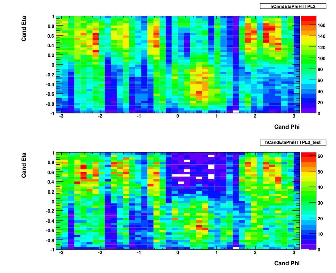
The above plots show 2-d histograms of eta and phi for pion candidates. The plot on the top shows the candidates from the production L2-G trigger. The plot on the bottom shows the eta and phi distribution for candidates from the L2-G 'test' trigger. As of May 2007, I am not using these to exclude any runs. I used Frank's pion trees to make these plots, imposing the following cuts on any pion candidate:
- Energy > 0.1 GeV
- PT > 5.0 GeV
- Asymmetry < .8
- Mass between .08 and .25 GeV
- No charged track association.
- BBC Timebin = 7,8 or 9.
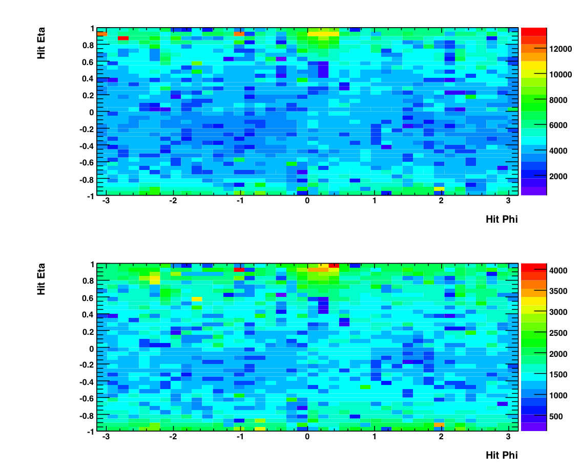
The above plot shows histograms of the eta and phi positions of individual photons (hits). Again the top plot shows photons from events from the production L2-G trigger while the bottom shows photons from the 'test' L2-G trigger. Note the lack of structure in these plots compared to the candidate plots. This is due to the SMD, which is used in making the top plots (i.e. a candidate needs to have good SMD information) and unused in the bottom plots (a hit does not reference the SMD.) The status tables for different fill periods can be found at the bottom of this page. You can see that there are some gaps in the smd which could be responsible for the structure in the Candidate plot.
Event Ratios

This plot shows, as a function of run number, the number of L2-G triggered events divided by the number of minbias triggers (w/ prescale.) This shows all the runs, before any outliers are removed.

This plot above shows a the histograms of the top plots. There is some subtlety here (as you have probably noticed) in that the data needs to be analyzed in four sets. The largest set (corresponding to the top left histogram) is all of the L2-G triggers from the 'production' level data, which consists of all the runs after ~100. The other three sets are all subsets of the 'test' status (i.e. the first ~100 runs) and reflect changes in the prescale and threshold levels. The characteristics from each subset are noted below.
Runs 3 -14 (top right):
Initial test thresholds
Prescale = 1
Runs 23 - 44 (lower left):
Higher thresholds (?)
Prescale = 2
Runs 45 - 93 (lower right):
Lower thresholds
Prescale = 1
Runs 93+ (top left):
Final thresholds (5.2 GeV)
Prescale = 1

The above plot shows the event ratio after outliers have been removed. To identify these outliers I took a four-sigma cut around the mean for each of the four histograms shown above, and removed any runs that fell outside this cut. The list of outlying runs and thier characteristics can be found here.
Pion Number


On the left are two plots showing the number of pions per triggered event (L2-G trigger) as a function of run index. The top plot is for all of the runs when the L2-G trigger had production status, while the bottom plot exhibits the runs for which the L2-G trigger had 'test' status (about the first 100 runs or so.) On the right are histograms of these two plots. To remove outliers from the runlist, I made a two-sigma cut around the mean of these histograms and removed any run that fell outside this range. Below are plots showing pion number per triggered event after the outlying runs have been removed. Note the change in scale from the original. A list of excluded runs and thier properties can be found here.

As you can see, there is some funny structre in the above plot. It's almost bi(or tri)-modal, with the mean number of pions per trigger jumping between .06 and .08 (or even .1). I think this is a consequence of the SMD. See below.

The above is a plot of the number of triggered photons that have GOOD SMD status normalized by the total number of triggered photons, as a function of run number. While this is crude, it gives an approximate measure of the percent of active SMD strips in the barell for each run. As you can see, the peaks and vallys in this plot mirror the peaks and vallys in pion yield above. Since the SMD is not required to satisfy the trigger but IS required to reconstruct a pion, we would expect that the pion reconstruction efficiency would decrease as the number of active SMD strips decreases. Indeed this is what appears to be happening.
I used Frank's pion trees to make these plots, imposing the following cuts on any pion candidate:
- Photon Et > 0.1 GeV
- PT > 5.2 GeV
- Asymmetry < .8
- Mass between .08 and .25 GeV
- No charged track association.
- BBC Timebin = 6, 7, 8, or 9.
- 'Good' SMD status.
Pion Yields
currently not in useSingle Spin Asymmetries
Run By Run
Runs are indexed from the beginning of the long-2 period. For reference, take a look at this file.

By Transverse Momentum


Tower and SMD info
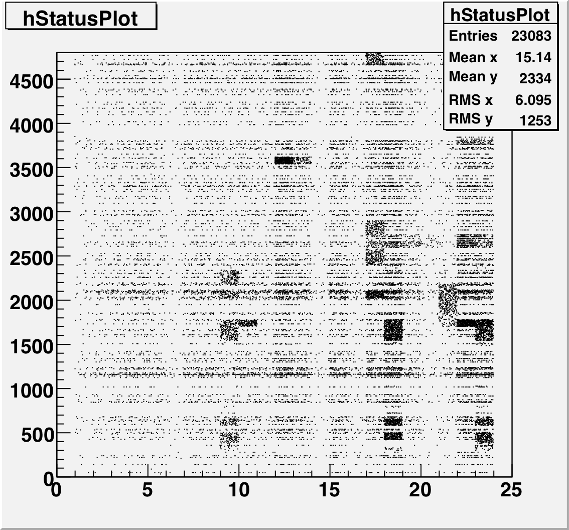
This is a plot of the tower status as a function of relative day (since the start of the second longitudinal period.) The 4800 towers are on the Y-Axis and Days are on the X axis. A dot means that that tower had a status other than good during that time period.
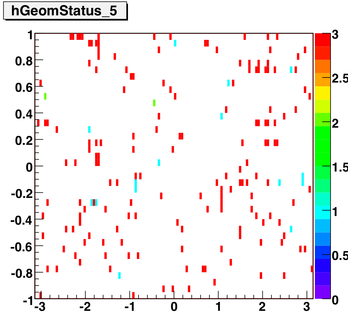
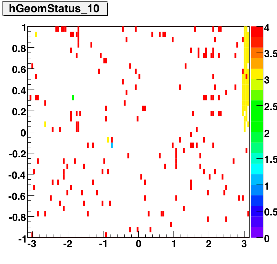
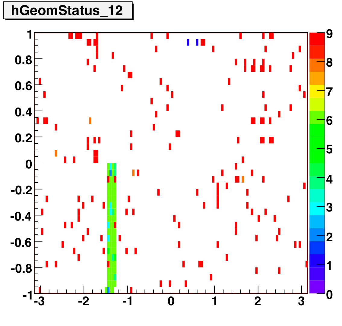
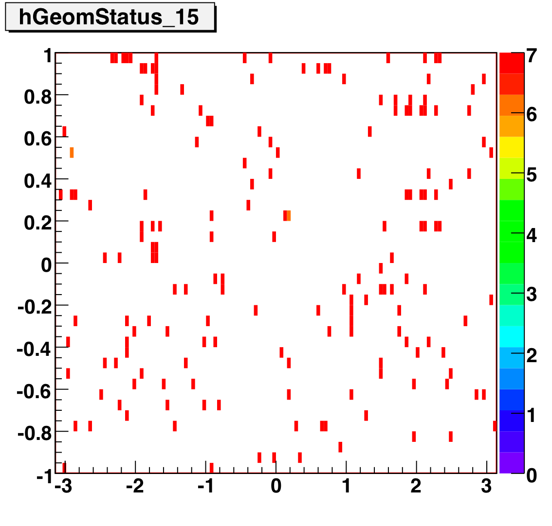
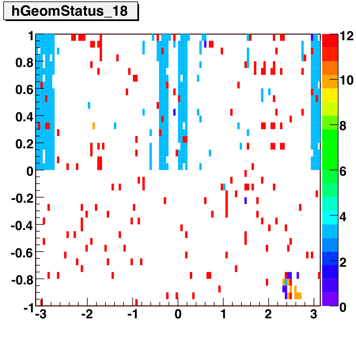
Tower Status Geometry
The below plots show the status as a function of phi and eta for different days representing different status periods. The title of the histogram refers to the relative day in the second longitudinal period (e.g. hGeomStatus_5 is for the fifth day of long-2.) The x and y axes correspond to detector phi and eta, and any space that is not white is considered a 'bad' tower. As you can see, for most of the barell for most of the time, most of the towers are good. Only for specific day ranges are there chunks of the barrel missing.
SMD Status
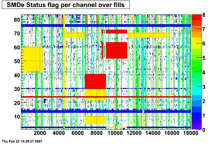
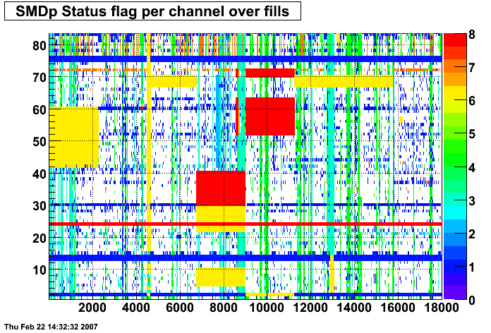
These two plots were made by Priscilla and they show the SMD status flags for SMD strips vs. Fill number. In these plots the strip number is plotted along the X-axis and the fill index number is plotted along the Y-Axis. Priscilla's fill index list can be found here. The important range for my particular analysis (i.e. the second longitudinal range) runs between fill indices 41 - 74. For my analysis I ignore any SMD strip that has a status other than good (== 0).
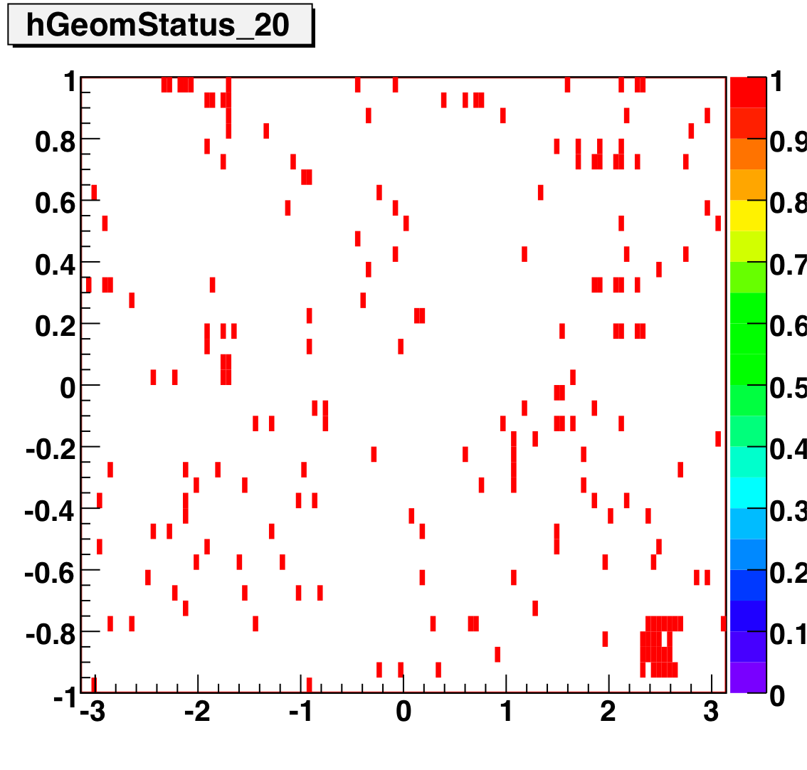
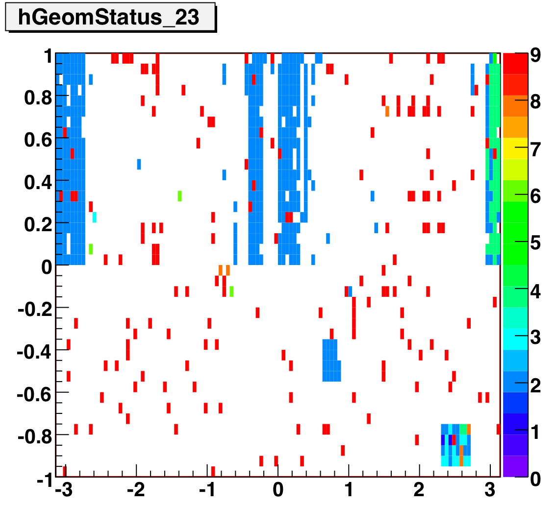
SMD Status Geometry
The plots below show the smd status as a function of geometry. The location of the strip in eta-phi space (w/ phi on the x axis and eta on the y axis.) You can see the eta and phi strip planes for four different fills (representative of different configurations) 7855, 7891, 7921, and 7949. Using Priscilla's iindexing these fills correspond to fills 46, 57, 68, and 72 in the above plots. We can see that these runs mark the beginning of major changes in the status tables, and each plot below represents a relativley stable running period. For my analysis I consider any area that is not light blue (i.e. any area with status other than 1) to be bad. Please note the difference between the SMD geometry plots and the BTOW geometry plots, namely, in the SMD plots whitespace represents 'bad' strips, whereas in the BTOW plots whitespace represents 'good' towers. All plots below were made by Priscilla.
Z Vertex


The above left plot shows average z vertex as a function of run index for the L2-G trigger. The upper plot shows all runs for which the L2-G trigger had production status, while the lower plot shows the first ~100 runs, for which the L2-G trigger had test status. The above right plot shows a histogram of the points on the above left plot. These plots show the average z vertex for all the events in a run, that is, they are not limited to pion candidates (as in some of the other QA measures.)

this plot above shows the average z vertex of L2-G events as a function of run index, with outlying runs removed. To identify outying runs, I took a four-sigma cut around the mean of each histogram (showed top right) and excluded any run for which the average z vertex fell outside this cut. Currently, I separate the 'test' from 'production' runs for analysis of outlyers. It would not be hard to combine them if this is deemed preferable. A list of the excluded runs, with thier average z verex can be found here.
SPIN 2008 Talk for Neutral Pions
Hi all-
My Spin 2008 talk and proceedings can be found below.
Update:
v2 reflects updates based on comments from SPIN pwg and others
Spin PWG Meeting (2/22/07)
Statistics for Late Longitudinal Running- ~ 400 runs (7132001 - 7156028)
- ~ 6.2 million events
- ~ 170K Neutral Pions for HTTP L2 Gamma trigger
- ~ 80K Neutral Pions for HT2 Trigger
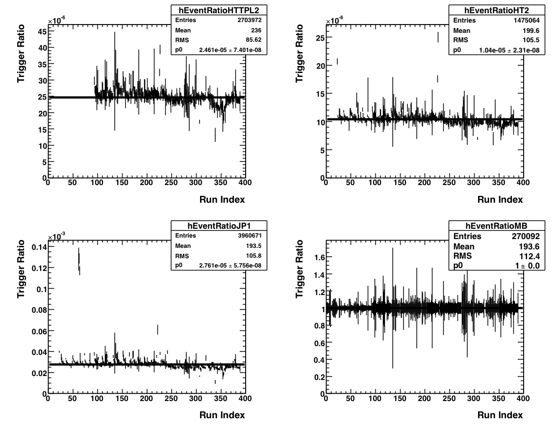
This plot shows, for the four triggers (HTTPL2, HT2, JP1, MB) the number of triggers registered normalized by the number of
minbias triggers registered, as a function of run index.
Pions per Event
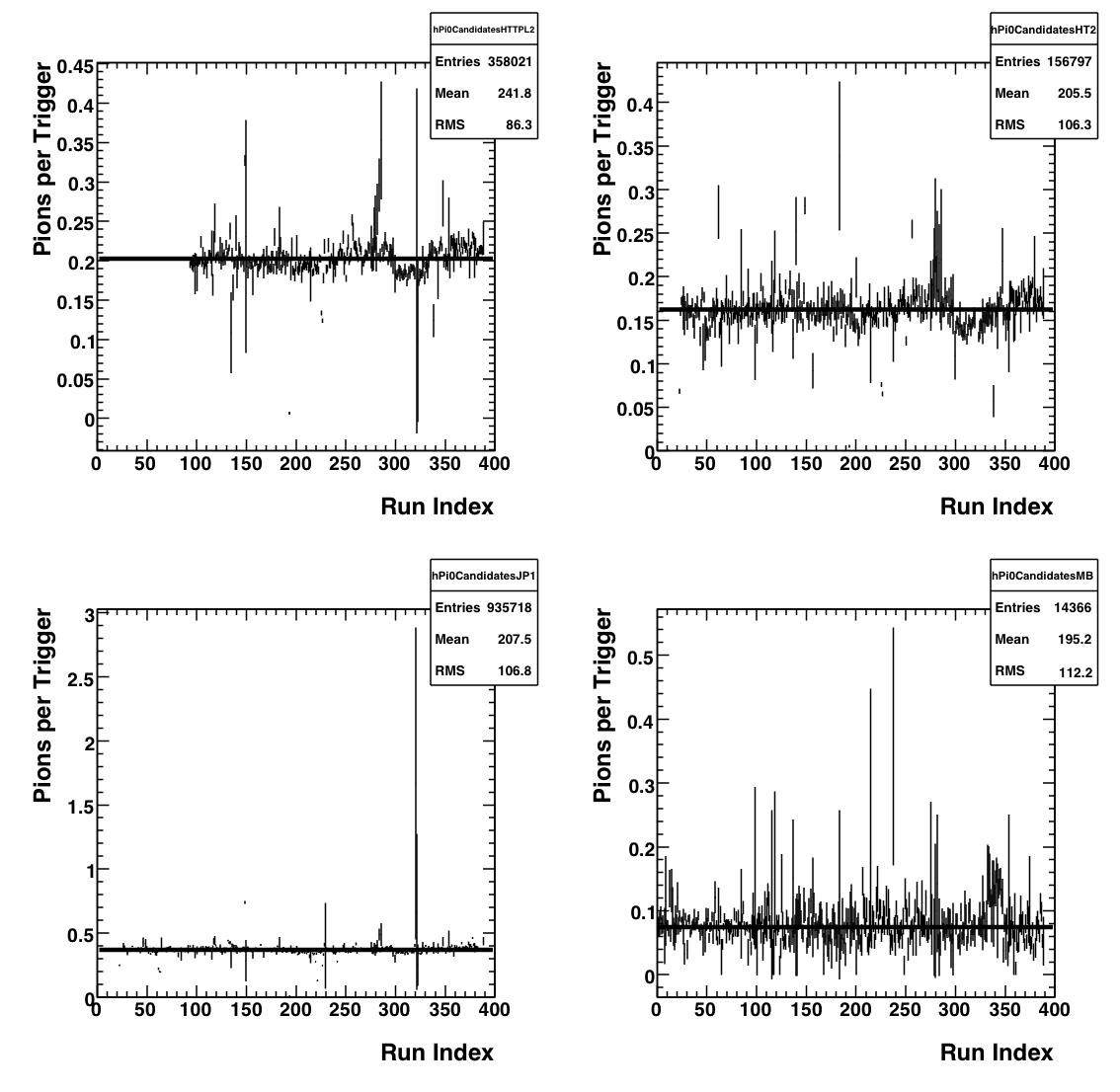
This plot shows the average number of neutral pions in an triggered event as a function of run number. For my purposes a
neutral pion consists of a reconstructed pion (using Frank's trees) that has the following cuts:
- Energy of each photon > 0.1 GeV
- Pt > 0.5 GeV
- Asymmetry < 0.8
- Mass between 0.08 and 0.25 GeV
- No charged track associated w/ the photons
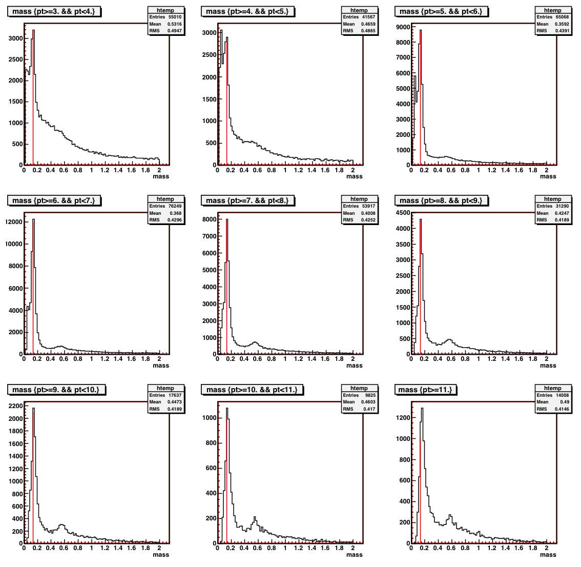
This plot shows the two-photon invariant mass spectrum for the HTTPL2-Gamma trigger, which is my most abundant and cleanest trigger. The mass
spectra are split into 1 GeV Pt bins, with the exception of the last one which is for everything with Pt more than 11 GeV.
Parsed Run List
Using the QA data shown on plots above (with more detail in my run QA page) I have come up with a preliminary 'good run list.' Basically I took the above event ratio and number ratio plots (along with a similar one for average z-vertex) and made a 4 sigma cut on either side the mean value. Any run with a value that fell outside this cut for either of the high tower triggers was excluded from my preliminary run list (right now the JP1 plots have no impact and are presented for curiosity sake.) Every run that passed these three tests was labeled 'good' and included in my list. My list and the associated run indexes can be found here. The list contains 333 runs.
ALL Checklist
The following is a checklist of 'to do' tasks toward a preliminary ALL measurement.
- Relative luminosity data for the late-longitudinal runs
- Polarization data (note, I have the numbers for the fast-offline CNI measurements and am refining the data for release.)
- Decisions on details (Pt binning, final mass window, etc.)
- Montecarlo studies
- Background studies
- Studies of other systematic effects.
- Other?
Spin PWG meeting (2/12/09)
The PDF for my slides is linked below.
Towards a Preliminary A_LL
Links for the 2006 Neutral Pion A_LL analysis
The numbered links below are in 'chronological' type order (i.e. more or less the order in which they should be looked at.) The 'dotted' links below the line are a side-effect in Drupal that lists all daughter pages in alphebetical order. They are the exact same as the numbered links and probably should just be ignored.
1. Run List QA
4. Cuts etc.
6. Invariant Mass Distribution
10. Sanity Checks
11. DIS Presentation
A_LL
The measurement of ALL for inclusive neutral pion production is seen below along with statistical error bars and a systematic error band. This asymmetry was calculated using a class developed by Adam Kocoloski (see here for .cpp file and here for .h file.) Errors bars are statistical only and propagated by ROOT. The gray band below the points represents the systematic uncertainties as outlined here. The relative luminosities are calculated on a run by run basis from Tai's raw scalar counts. Each BBC timebin is treated seperately. The theory curves are GRSV predictions from 2005. These will change slightly for 2006.

Bin ALL (x10-2)
1 0.80 +/- 1.15
2 0.58 +/- 1.36
3 2.03 +/- 1.89
4 -0.84 +/- 3.06
Cuts and Parameters
Here I will detail the some general information about my analysis; topics that aren't substantial enough to warrant their own page but need to be documented. I will try to be as thorough as I can.
Data
Run 6 PP Long 2 Only.
Run Range: 7131043 - 7156040
Fill Range: 7847 - 7957
Days: 131 - 156 (May 11 - June 5, 2006)
HTTP L2gamma triggered data (IDs 5, 137611)
Trees using StSkimPionMaker (found in StRoot/StSpinPool/) and Murad's spin analysis chain macro
Trees located in /star/institutions/mit/ahoffman/Pi0Analysis/Murads_Production_1_08/
Cluster Finding Conditions
Detector Seed Add
BEMC 0.4 GeV 0.05 GeV
SMDe/p 0.4 GeV 0.005 GeV
Pion Finding Cuts
Event passes online and software trigger for L2gamma
Energy asymmetry (Zgg) <= 0.8
Charged track veto (no photon can have a charged track pointing to its tower)
BBC timebins 6,7,8,9 (in lieu of a z vertex cut)
At least one good SMD strip exists in each plane
-0.95 <= eta <= .95
Z vertex found
Pt Bins for ALL
All reconstructed pion candidates are separated by Pt into four bins:
5.20 - 6.75
6.75 - 8.25
8.25 - 10.5
10.5 - 16.0
Simulation
Full pythia (5 to 45 GeV/c in partonic Pt, weighted)
Single pion, photon, and eta simulations (2 - 25 GeV/c in particle Pt, unweighted)
EMC simulator settings:
15% Tower Spread
25% SMD Spread
SMD Max ADC: 700
SMD Max ADC spread: 70
(see this link for explanation of SMD Max ADC parameters)
Four representative timestamps used:
20060516, 062000 (40%)
20060525, 190000 (25%)
20060530, 113500 (25%)
20060603, 130500 (10%)
Full pythia trees located in /star/institutions/mit/ahoffman/Pi0Analysis/MC_Production_2_08/
Single particle trees located in /star/institutions/mit/ahoffman/Pi0Analysis/single_particle_simulations/
DIS 2008 Presentation
Below you will find a link to a draft my DIS 2008 presentation.
Energy Subtracted A_LL Calculation
For my single particle Monte Carlo studies, I argued (here) that I needed to add a small amount of energy to each reconstructed photon to better match the data. This small addition of energy brings the simulation mass distributions into better alignment with the mass distributions in the data. I did not, however, subtract this small bit of energy from reconstructed (data) pions. This affects ALL in that pion counts will migrate to lower Pt bins and some will also exit the low end of the mass windown (or enter the high end.) So I calculated ALL after subtracting out the 'extra' energy from each photon. The plot below shows the original ALL measurement in black and the new measurement in red.

The values from both histograms are as follows:
Bin black (orig) red (new)
1 .0080 .0095
2 .0058 .0092
3 .0203 .0196
4 -.0084 -.0069
So things do not change too much. I'm not sure which way to go with this one. My gut tells me to leave the data alone (don't correct it) and assign a systematic to account for our lack of knowledge of the 'true' energy of the photons. The error would be the difference between the two plots, that is:
Bin Sys. Error (x10-3)
1 1.5
2 3.4
3 0.7
4 1.5
Integral Delta G Study
Using Werner's code I calculated A_LL for pi0 production over my eta range for 15 different integral values of Delta G. Below I plot the measured A_LL points and all of those curves.
I then calculated chi^2 for each of the curves. Below is the chi^2 vs. integral delta g.
The red line shoes minimum chi^2 + 1. For my points, GRSV-Std exhibits the lowest chi^2, but GRSV-Min is close. My data indicates a small positive integral value of delta g in the measured x range.
Invariant Mass Distribution
The two-photon invariant mass distribution can be roughly broken up into four pieces, seen below*.
Fig. 1

The black histogram is the invariant mass of all pion candidates (photon pairs) with pt in the given range. I simulate each of the four pieces in a slightly different way. My goal is to understand each individual piece of the puzzle and then to add all of them together to recreate the mass distribution. This will ensure that I properly understand the backgrounds and other systematic errors associated with each piece. To understand how I simulate each piece, click on the links below.
1. Pion Peak
2. Eta Peak
Once all of the four pieces are properly simulated they are combined to best fit the data. The individual shapes of are not changed but the overall amplitude of each piece is varied until the chisquared for the fit is minimized. Below are plots for the individual bins. Each plot contains four subplots that show, clockwise from upper left, the four individual peices properly normalized but not added; the four pieces added together and compared to data (in black); the ratio of data/simulatio histogramed for the bin; and a data simulation comparison with error bars on both plots.
Bin 1: 5.2 - 6.75 GeV/c

Bin 2: 6.75 - 8.25 GeV/c

Bin 3: 8.25 - 10.5

Bin 4: 10.5 - 16.0

Below there is a table containing the normalization factors for each of the pieces for each of the bins as well as the total integrated counts from each of the four pieces (rounded to the nearest whole count.)
| bin | low norm. | low integral | pion norm. | pion integral | eta norm. | eta integral | mixed norm. | mixed integral |
| 1 | 121.3 | 9727 | 146.4 | 75103 | 20.91 | 5290 | 0.723 | 44580 |
| 2 | 77.34 | 4467 | 77.81 | 51783 | 20.86 | 6175 | 0.658 | 34471 |
| 3 | 40.13 | 3899 | 29.41 | 23687 | 12.93 | 6581 | 1.02 | 18630 |
| 4 | 5.373 | 1464 | 5.225 | 8532 | 2.693 | 3054 | 0.521 | 6276 |
Table 2 below contains, for each source of background, the total number of counts in the mass window and the background fraction [background/(signal+background)].
| Bin | Low Counts | Low B.F (%) | Eta Counts | Eta B.F (%) | Mixed Counts | Mixed B.F (%) |
| 1 | 2899 | 3.60 | 1212 | 1.50 | 4708 | 5.84 |
| 2 | 2205 | 3.96 | 917 | 1.65 | 3318 | 5.96 |
| 3 | 2661 | 9.29 | 633 | 2.21 | 1507 | 5.26 |
| 4 | 858 | 8.56 | 170 | 1.70 | 591 | 5.89 |
* Note: An astute observer might notice that the histogram in the top figure, for hPtBin2, does not exactly match the hPtBin2 histogram from the middle of the page (Bin 2.) The histogram from the middle of the page (Bin 2) is the correct one. Fig. 1 includes eta from [-1,1] and thus there are more total counts; it is shown only for modeling purposes.
Combinatoric Background
The last piece of the invariant mass distribution is the combinatoric background. This is the result of combining two non-daughter photons into a pion candidate. Since each photon in an event is mixed with each other photon in an attempt to find true pions, we will find many of these combinatoric candidates. Below is a slide from a recent presentation describing the source of this background and how it is modeled.
---------------------------------------

-------------------------------------------
As it says above we take photons from different events, rotate them so as to line up the jet axes from the two events, and then combine them to pion candidates. We can then run the regular pion finder over the events and plot out the mass distribution from these candidates. The result can be seen below.

These distributions will be later combined with the other pieces and normalized to the data. For those who are interested in the errors on these plots please see below.

Eta Peak
I treat the eta peak in a similar way as the pion peak. I throw single etas, flat in Pt from 2 - 25, and reconstruct the two-photon invariant mass distribution for the results. The thrown etas are weighed according to the PHENIX cross-section as outlined here. The mass distributions for the four pt bins can be seen below. (I apologize for the poor labeling, the x-axis is Mass [GeV/c^2] and the y-axis is counts.) Don't worry about the scale (y-axis.) That is a consequence of the weighting. The absolute scale will later be set by normalizing to the data.

These plots will later be combined with other simulations and normalized to the data. The shape will not change. For those interested in the errors, that can be seen below.

Low Mass Background
The low mass background is the result of single photons being artifically split by the detector (specifically the SMD.) The SMD fails in it's clustering algorithm and one photon is reconstructed as two, which, by definition, comprises a pion candidate. These will show up with smaller invariant masses than true pions. Below is a slide from a recent presentation that explaines this in more detail and with pictures.
----------------------------------

----------------------------------
We can reproduce this background by looking at singly thrown photons and trying to find those that are artificially split by the clustering algorithm. Indeed when we do this, we find that a small fraction (sub 1%) do indeed get split. We can then plot the invariant mass of these pion candidats. The results can be seen below. (x-axis is mass in GeV/c^2.)

These mass distributions will later be combined with other pieces and normalized to the data. For those interested in the errors on these histograms please see below.

Pion Peak
To study the pion peak section of the invariant mass distribution I looked at single pion simulations. The pions were thrown with pt from 2 - 25 GeV/c flat and were reconstructed using the cuts and parameters described in the cuts, etc. page. The mass of each reconstructed pion is corrected by adding a small amount of energy to each photon (as outlined here.) After this correction the peak of the reconstructed mass distribution is aligned with the peak of the data. The mass distributions from the four bins can be seen below.

Later, these peaks will be normalized, along with the other pieces, to the data. However, the shape will not change.
If you are interested in seeing the errors on the above plots, I reproduce those below.

Polarization
I am using the final polarization numbers from run 6, released by A. Bazilevsky to the spin group on December 4, 2007. The files can be found below.
Pt Dependent Mass
The two-photon invariant mass is given (in the lab frame) by
M = Sqrt(2E1E2(1 - Cos(theta)))
where E1 and E2 are the energies of the two photons and theta is the angle between those photons. For every real photon we should measure ~135 MeV, the rest mass of the pi0. Of course, the detectors have finite resolution and there is some uncertainty in our measurement of each of the three quantities above, so we should end up measuring some spread around 135 MeV.
But it is not that simple. We do not see a simple spread around the true pion mass. Instead, we see some pt dependence in the mean reconstructed mass.


The above left plot shows the two-photon invariant mass distribution separated into 1 GeV bins. The pion peak region (between ~.1 and .2 GeV) has been fit with a gaussian. The mean of each of those gaussians has been plotted in the above right as a function of Pt. Obviously the mean mass is increasing with Pt. This effect is not particularly well understood. It's possible that the higher the Pt of the pion, the closer together the two photons will be in the detector and the more likely it is that some of the energy from one photon will get shifted to the other photon in reconstruction. This artificially increases the opening angle and thus artificially increases the invariant mass. Which is essentially to say that this is a detector effect and should be reproducible in simulation. Indeed...

The above plot overlays (in red) the exact same measurement made with full-pythia monte carlo. The same behavior is exhibited in the simulation. Linear fits to the data and MC yield very similar results...
-- M = 0.1134 + 0.0034*Pt (data)
-- M = 0.1159 + 0.0032*Pt (simulation)
If we repeat this study using single-particle simulations, however, we find some thing slightly different.

-- M = 0.1045 + 0.0033*Pt
So even in single-particle simulation we still see the characteristic rise in mean reconstructed mass. (This is consistent with the detector-effect explanation, which would be present in single-particle simulation.) However, the offset (intercept) of the linear fit is different. These reconstructed pions are 'missing' ~11 MeV. This is probably the effect of jet background, where other 'stuff' in a jet get mixed in with the two decay photons and slightly boost their energies, leading to an overall increase in measured mass.
The upshot of this study is that we need to correct any single-particle simulations by adding a slight amount of extra energy to each photon.
Relative Luminosity
For my relative luminosity calculations I use Tai's relative luminosity file that was released on June 14th, 2007.
I read this using the StTamuRelLum class, which, given a run number and BBC timebin, reads in the raw scalar values for each spinbit. Each event is assigned raw scalar counts for each spinbit and every event from the same run with the same timebin should have the same scalar counts assigned. When it comes time to calculate my asymmetry, the relative luminosity is calculated from these scalar counts.
Run List
Below you will find the runlist I used for all of the studies leading up to a preliminary result. For a more detailed look at how I arrived at this runlist please see my run QA page.
Sanity Checks
Below there are links to various 'sanity' type checks that I have performed to make sure that certain quantities behave as they should
Mass Windows
The nominal mass window was chosen 'by eye' to maximize the number of pion candidates extracted while minimizing the backgrounds (see yield extraction page.) I wanted to check to see how this choice of mass window would affect the measurement of ALL. To this end, ALL was calculated for two other mass windows, one narrower than the nominal window (.12 - .2 GeV) and one wider than the nominal window (.01 - .3 Gev). The results are plotted below where the nominal window points are in black, the narrow window points are in blue and the wide window points are in red. There is no evidence to indicate anything more than statistical fluctuations. No systematic error is assigned for this effect.

Revised Eta Systematic
After some discussion in the spin pwg meeting and on the spin list, it appears I have been vastly overestimating my eta systematic as I was not properly weighing my thrown single etas. I reanalyzed my single eta MC sample using weights and I found that the background contribution from etas underneath my pion peak is negligible. Thus I will not assign a systematic error eta background. The details of the analysis are as follows. First I needed to assign weights to the single etas in my simulation. I calculated these weights based on the published cross section of PP -> eta + X by the PHENIX collaboration (nucl-ex 06110066.) These points are plotted below. Of course, the PHENIX cross section on reaches to Pt = 11 GeV/c and my measurement reaches to 16 GeV/c. So I need to extrapolate from the PHENIX points out to higher points in Pt. To do this I fit the PHENIX data to a function of the form Y = A*(1 + (Pt)/(Po))^-n. The function, with the parameters A = 19.38, P0 = 1.832 and n = 10.63, well describes the available data.

I then caluclate the (properly weighted) two-photon invariant mass distribution and calculate the number of etas underneath the pion peak. The eta mass distributions are normalized to the data along with the other simulations. As expected, this background fraction falls to ~zero. More specifically, there was less than ten counts in the signal reigon for all four Pt bins. Even considering a large background asymmetry (~20%) this becomes a negligable addition to the total systematic error. The plots below show the normalized eta mass peaks (in blue) along with the data (in black.) As you can see, the blue peaks do not reach into the signal reigion.

Unfortunately, the statistics are not as good, as I have weighted-out many of the counts. I think that the stats are good enough to show that Etas do not contribute to the background at any significant level. For the final result I think I would want to spend more time studying both single particle etas and etas from full pythia.
I should also note that for this study, I did not have to 'correct' the mass of these etas by adding a slight amount of energy to each photon. At first I did do this correction and found that the mass peaks wound up not lining up with the data, When I removed the correction, I found the peaks to better represent the data.
In summary: I will no longer be assigning a systematic from eta contamination, as the background fraction is of order 0.01% and any effect the would have on the asymmetry would be negligible.
Single Spin Asymmetries
The plots below show the single spin asymmetries (SSA) for the blue and yellow beams, as a function of run index. These histograms are then fit with flat lines. The SSA's are consistent with zero.


Systematics
We need to worry about a number of systematic effects that may change our measurement of ALL. These effects can be broadly separated into two groups: backgrounds and non backgrounds. The table below summarizes these systematic errors. A detailed explanation of each effect can be found by clicking on the name of the effect in the table.
| Systematic Effect | value {binwise} (x10-3) |
| Low Mass Background | {1.0; 1.1; 3.8; 1.0} |
| Combinatoric Background | {1.0; 0.86; 1.6; .03} |
| Photon energy Uncertainty | {1.5; 3.4; 0.7; 1.5} |
| Non Longitudinal Components* | 0.94 |
| Relative Luminosity* | 0.03 |
| Total** | {2.3; 3.8; 4.3; 2.0} |
* These numbers were taken from the Jet Group
** Quadrature sum of all systematic errors
Alternate Calculation of Eta Systematic
At the moment I am calculating the systematic error on ALL from the presence of Etas in the signal reigon using theoretical predictions to estimate ALLeta. The study below is an attempt to see how things would change if I instead calculated this systematic from the measured ALLeta. Perhaps, also, this would be a good place to flesh out some of my original motivation for using theory predictions.
First order of buisness is getting ALLeta. Since this was done in a quick and dirty fashion, I have simply taken all of my pion candidates from my pion analysis and moved my mass window from the nominal pion cuts to a new window for etas. For the first three bins this window is .45 GeV/c2 < mass < .65 GeV/c2 and for the fourth bin this is .5 GeV/c2 < mass < .7 GeV/c2. Here is a plot of ALLeta, I apologize for the poor labeling.

I guess my first reason for not wanting to use this method is that, unlike the other forms of background, the Etas A_LL ought to be Pt dependent. So I would need to calculate the systematic on a bin-by-bin basis, and now I start to get confused because the errors on these points are so large. Should I use the nominal values? Nominal values plus one sigma? I'm not sure.
For this study I made the decison to use ALLtrue as the values, where ALLtrue is calculated from the above ALL using the following formula:
ALLM = (ALLT + C*ALLBkgd)/(1 + C)
Remembering that a large portion the counts in the Eta mass window are from the combinatoric background. I then calculate the background fraction or comtamination factor for this background (sorry I don't have a good plot for this) and get the following values
Bin Bkg fraction
1 77.2%
2 60.9%
3 44.6%
4 32.6%
Plugging and chugging, I get the following values for ALLtrue:
Bin ALLT
1 .0298
2 .0289
3 -.0081
4 .175
Using these values of ALL to calculate the systematic on ALLpion I get the following values:
Bin Delta_ALLpion (x10^-3)
1 .33
2 .38
3 .63
4 3.1
Carl was right that these values would not be too significant compared to the quad. sum of the other systematics, except for final bin which becomes the dominant systematic. In the end, I would not be opposed to using these values for my systematic *if* the people think that they tell a more consistent story or are easier to justify/explain than using the theory curves. (i.e. if they represent a more accurate description of the systematic.)
Combinatoric Systematic
For the combinatoric background systematic we first estimate the background contribution (or contamination factor) to the signal reigon. That is we integrate our simulated background to discern the precentage of the signal yield that is due to background counts. The plots below show, for each of the four bins, the background fraction underneath the singal peak. The background (simulation) is in green and the signal (data) is in black and the background that falls in the signal reigon is filled-in with green.

The background fractions for the bins are
Bin 1: 6.1%
Bin 2: 6.1%
Bin 3: 5.7%
Bin 4: 6.2%
Then I consider how much this background fraction could affect my measured asymmetry. So I need to meausre the asymmetry in the high-mass reigon. I do this, taking the mass window to be 1.2 to 2.0 GeV/c2. I do not expect this asymmetry to be Pt-dependant, so I fit the asymmetry with a flat line and take this to be the asymmetry of the background, regardless of Pt. The plot below shows this asymmetry and fit.

Finally, I calculate the systematic error Delta_ALL = ALLTrue - ALLMeasured where:
ALLM = (ALLT + C*ALLBkgd)/(1 + C)
And C is the background fraction. This yields in the end as a systematic error (x10-3):
Bin 1: 1.0
Bin 2: 0.9
Bin 3: 1.6
Bin 4: 0.03
Eta Systematic
For the eta background systematic we first estimate the background contribution (or contamination factor) to the signal reigon. That is we integrate our simulated background to discern the precentage of the signal yield that is due to background counts. The plots below show, for each of the four bins, the background fraction underneath the singal peak. The background (simulation) is in blue and the signal (data) is in black and the background that falls in the signal reigon is filled-in with. Below that is the same four plots but blown up to show the contamination.

Here we blow up these plots

The background fractions for the bins are
Bin 1: 1.50%
Bin 2: 1.65%
Bin 3: 2.21%
Bin 4: 1.70%
Then I consider how much this background fraction could affect my measured asymmetry. So I need to measure the asymmetry in the etas. So instead of measuring the asymmetry in the etas I will use a theoretic prediction for ALL. From GRSV standard and GRSV min I approximate that the size of ALL in my Pt range to be between 2 - 4%.

I stole this plot from C. Aidala's presentation at DNP in Fall 2007. Since GRSV-Max is ruled out by the 2006 jet result I restrict myself only to min, standard and zero. For a conservative estimate on the systematic, I should pick, for each Pt bin, the theory curve that maximizes the distance between the measured and theoretical asymmetries. Unfortunately, at this time I do not have predictions for Pt above 8, so I must extrapolate from this plot to higher bins. For the first two bins this maximum distance would correspond to GRSV standard (ALLbg ~ 0.02). For the third bin, this would correspond to GRSV = 0 (ALLbg ~ 0.). For the fourth bin (which has a negative measured asymmetry) I extrapolate GRSV standard to ~4% and use this as my background ALL.
Systematic (x10-3)
Bin 1: 0.18
Bin 2: 0.23
Bin 3: 0.43
Bin 4: 0.82
Low Mass Systematic
For the low mass background systematic we first estimate the background contribution (or contamination factor) to the signal reigon. That is we integrate our simulated background to discern the precentage of the signal yield that is due to background counts. The plots below show, for each of the four bins, the background fraction underneath the singal peak. The background (simulation) is in red and the signal (data) is in black and the background that falls in the signal reigon is filled-in with red.

The background fractions for the bins are
Bin 1: 3.5%
Bin 2: 4.2%
Bin 3: 9.3%
Bin 4: 8.3%
Then I consider how much this background fraction could affect my measured asymmetry. So I need to meausre the asymmetry in the low-mass reigon. I do this, taking the mass window to be 0 to 0.7 GeV/c2. I do not expect this asymmetry to be Pt-dependant, so I fit the asymmetry with a flat line and take this to be the asymmetry of the background, regardless of Pt. The plot below shows this asymmetry and fit.

Finally, I calculate the systematic error Delta_ALL = ALLTrue - ALLMeasured where:
ALLM = (ALLT + C*ALLBkgd)/(1 + C)
And C is the background fraction. This yields in the end as a systematic error (x10-3):
Bin 1: 1.0
Bin 2: 1.1
Bin 3: 3.7
Bin 4: 1.1
Yield Extraction
After all the pion candidates have been found and all the cuts applied, we need to extract the number of pions in each bin (in each spin state for ALL.) To do this we simply count the number of pion candidates in a nominal mass window. I chose the mass window to try to maximize the signal region and cut out as much background as possible. For the first three Pt bins, this window is from .08 - .25 GeV/c2 and in the last bin the window is from .1 - .3 GeV/c2. The window for the last Pt bin is shifted mostly to cut out more of the low mass background and to capture more pions with higher than average reconstructed mass. The windows can be seen below for bins 2 and 4.


These Pt bins are broken down by spin state, and the individual yields are reported below.
| Bin | uu | du | ud | dd | Total |
| 1 | 20209 | 20088 | 19961 | 20231 | 80489 |
| 2 | 14088 | 14057 | 13645 | 13825 | 55615 |
| 3 | 7224 | 7080 | 7107 | 7204 | 28615 |
| 4 | 2505 | 2470 | 2552 | 2491 | 10018 |
Tower By Tower Pion Peaks
Calibration
I am trying to calibrate the BEMC using neutral pions. As of now I am only using the L2 Gamma trigger for the second longitudinal running period, although I plan on incorporating the transverse data as well since the calibration should be the same for the two running periods. The procedure, so far, is listed below. Items 1 - 4 have been done for the long2 data set and are not difficult. Items 5+ I have not done yet, nor am I certain if they are the correct way to proceed.
1. Find all pion candidates using Frank's finder.
2. Calculate the mass for each di-photon pair.
3. Find the tower struck by each photon in the candidate and fill that tower's histogram with the invariant mass of the pion candidate. Note that if the two photons strike two different towers, both towers are filled with the mass of one pion.
4. Fit the towers with a gaussian + linear function and extract the location of the peak (see below.)
* * *
5. Using the mass peaks, calculation a correction factor for each tower, and apply this correction factor to the tower response (gains? I'm not sure.)
6. Repeat until desired level of precision is reached.
Plots
Good Tower:

Poor Statistics (Hope to improve w/ Transverse):

Poor Fit:

Spiked Fit (Chi^2 = 60/32 if you can't read it.)

A .pdf with all 4800 towers, and their fits can be found here. It is about 50 MB.