TPC
FCF
Please attach any information about the Fast Cluster Finder (FCF) here.
Cluster flags
I am sending a short description of the
TPX cluster finder flags. This is more an Offline issue
but I guess this is a better group since it is a bit
technical.

1) The flags are obtained in the same way other
variables such as timebin and pad are obtained.
I understand that this is not exported to StHit *shrug*.

See i.e. StRoot/RTS/src/RTS_EXAMPLE/rts_example.C

2) They are defined in:

StRoot/RTS/src/DAQ_TPX/tpxFCF.h

The ones pertaining to Offline are:

FCF_ONEPAD           This cluster only had 1 pad.
Generally, this cluster should be ignored unless
you are interested in the prompt hits where this
might be valid. The pad resolution is poor, naturally.

FCF_MERGED           This is a dedconvoluted cluster.
The position and charge have far larger errors
than normal clusters.

FCF_BIG_CHARGE    The charge was larger than 0x7FFF so
the charge precision is lost. The value is OK but the precision is
1024 ADC counts. Good for tracking, not good for dE/dx.

FCF_BROKEN_EDGE       This is the famous row8 cluster.
Flag will disappear from valid clusters
once I have the afterburner running.

FCF_DEAD_EDGE          Garbage and should be IGNORED!
This cluster touches either a bad pad or an end
of row or is somehow suspect. I need this flag for internal debugging
but the users should IGNORE those clusters!

        -- Tonko
I commited the "padrow 8" afterburner to the DAQ_TPX
CVS directory. If all runs well, you should see no more
peaks on padrow 8. The afteburner runs during the
DAQ_READER unpacking.

However, please pay attention to the cluster finder flags
which I mentioned in an email ago. Specifically:

"FCF_DEAD_EDGE          Garbage and should be IGNORED!
This cluster touches either a bad pad or an end
of row or is somehow suspect. I need this flag for internal debugging
but the users should IGNORE those clusters!"

         -- Tonko
Field Cage Shorts
This page is for information regarding shorts or current anomalies in the TPC field cages.
Excess current seen in 2006
The attached powerpoint file from Blair has plots of the excess current seen in the IFC East for 2006.
Modeled distortions
Modeling the Distortion
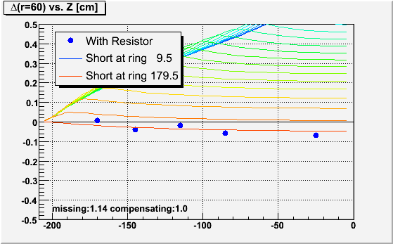
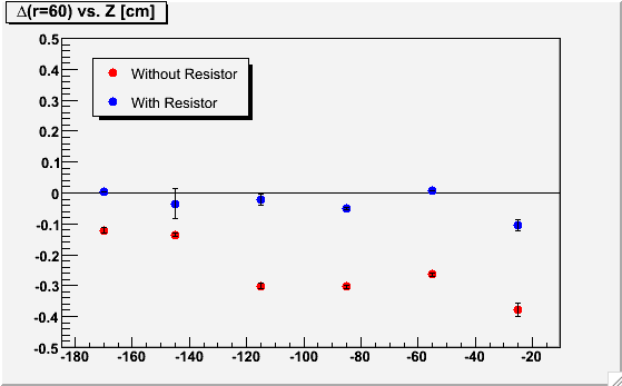
Using StMagUtilities, Jim Thomas and I were able to compare models of the distortions caused by shorts at specific rings in the IFC with the laser data. First, I'll have to say that I was wrong from my Observed laser distortions: the distortion to laser tracks does not have the largest slope at the point where the short is. Instead, it has a maximum at that point! The reason is that the z-component of the electric field due to the distortion (withouth compensating resistor) changes signs at the location of the short. So ExB also changes directions, and the TPC hits are distorted in one rPhi direction on the endcap side of the short, and in the opposite rPhi direction closer to the central membrane.This can be seen in the following plot, where I again show the distortion to laser tracks at a radius of 60cm (approximately the first TPC padrow) versus Z in the east TPC using distored run 7076029 minus undistorted run 7061100 as red data points. Overlayed are curves for the same measure from models of a half-resistor short (actually, 1.14 MOhm short as determined by the excess current of ~240+/-10nA [a full 2MOhm short equates to 420nA difference]) located at rings 9.5, 10.5, ..., 169.5, 179.5 (there are only 182 rings).
[note: earlier plots I have shown included laser data at Z = -55cm, but I've found that the laser tracks there weren't of sufficient quality to use; I've also tried to mask off places where lasers cross over each other]
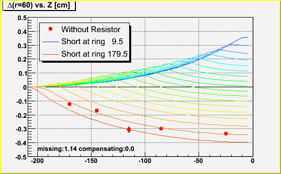
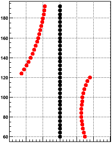
The above plot points towards a short which is located somewhere among rings 165-180 (Z < -190cm). As the previous years' shorted rings were rings 169 and 170 ( = short at ring 169.5), it seems highly likely that the present short is in the same place. More detail can be seen by looking at the actual laser hits. The first listed attached file shows the laser hits as a function of radius for lasers at several locations in Z. The dark blue line is a simple second order polynomial fit I used to obtain the magnitude of the distortion at radius 60cm, which I used in the above plot. The magenta line is the model of the half-resistor short at ring 169.5, and the light blue line is the same for ring 179.5 (the bottom two curves on the above plot). Either curve seems to match the radial dependence fairly well.
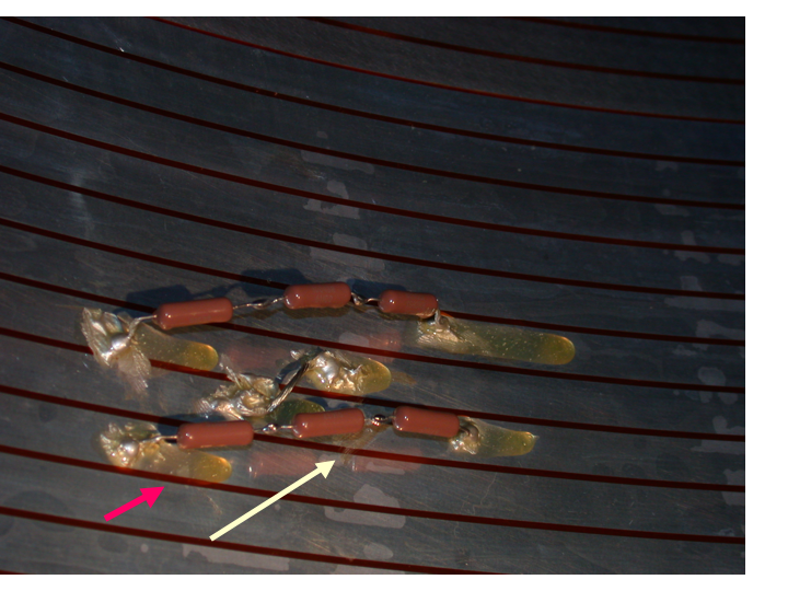
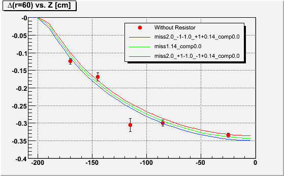
Further refinement can be achieved by modeling the exact resistor chain. We have a permanent short at ring 169.5 (rings 169 and 170 have been tied together), and have replaced the two 2MOhm resistors between 168-169 and 170-171 with two 3MOhm resistors (see the attached photo of the repair, with arrows pointing to candidate locations for shorts via drops of silver epoxy). So it is more likely that we have a 1.14MOhm short on one of these two 3 MOhm resistors. The three curves in this next plot are:
- red: 1.14MOhm short on a 3MOhm resistor at 168.5, full short at 169.5, 3MOhm resistor at 170.5
- green: 1.14MOhm short on a 2MOhm resistor at 169.5, normal 2.0MOhm resistors at 168.5 and 170.5
- blue: 3MOhm resistor at 168.5, full short at 169.5, 1.14MOhm short on a3MOhm resistor at 170.5
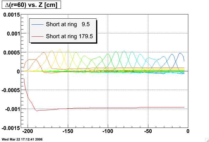
We can also take a look at the data with the resistor in. Here is the same plot as before with a 1.14MOhm short at the same locations, but with an additional compensating resistor of 1.0MOhm. The fact that all the data points are below zero points again towards a short near the very end of the resistor chain, preferring a location of perhaps 177.5 over shorts near ring 170. These plots do not include the use of the 3MOhm resistors, but that difference is below the resolution presented here.
Zoom in with finer granularity between rings (every other ring short shown):
The second listed attached file shows the laser hits as a function of radius for lasers at several locations in Z for the case of the resistor in, again with magenta and blue curves for the model with shorts at ring 169.5 and 179.5 respectively.
Applying the Correction
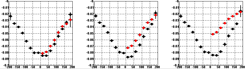
I tried running reconstruction on the lasers using the distortion corrections for the 1.14MOhm short at three locations: 170.5 and 171.5 (two possible spots indicated in Alexei's repair photo), and 175.5 (closer to what the with-resistor data pointed to). The results are in the following plots. The conclusion is that the 175.5 location seems to do pretty well at correcting the data, slightly better than the 170.5 and 171.5 locations, for both with and without compensating resistor. For this reason (the laser data), we will proceed with FastOffline using a short at 175.5, even though we have no strong reasons outside the laser data to suspect that the short is anywhere other than the rings 168-172 area where the fix was made.
| 170.5 | 171.5 | 175.5 |
|---|---|---|

|
|

|
Gene Van Buren
gene@bnl.gov
Choosing an external resistance for an IFC short
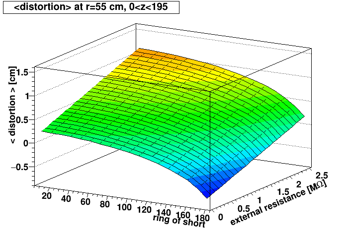
It is clear that when a field cage short is close to the endcap, it is best to add an external resistance to compensate for the amount of the missing resistance from the short as that would restore the current along the length of the resistor chain and only disrupt the potential at the last (outermost) rings instead of along the full length. A short near the central membrane would benefit less from this as restoring the proper current does restore the potential drop between each ring, but leaves almost all rings at a potential offset from the intended potential, essentially tilting the E field over nearly the whole volume.But the question then comes as to whether we can decide on the best external resistance for minimizing the distortion, to align with the principle that the best distortion we can choose is the one which requires the least correction, in case we're not quite correcting it accurately. To answer that, the distortion modeling was run with a variety of locations for an IFC west 2 MOhm single-resistor short, and a variety of external resistances. The code to run this modeling has been attached as a tar file to this Drupal page in case there is interest to re-run it (e.g. for an OFC short).
Here are the results:
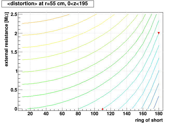
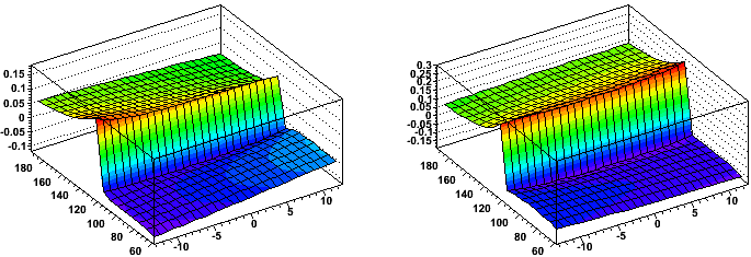
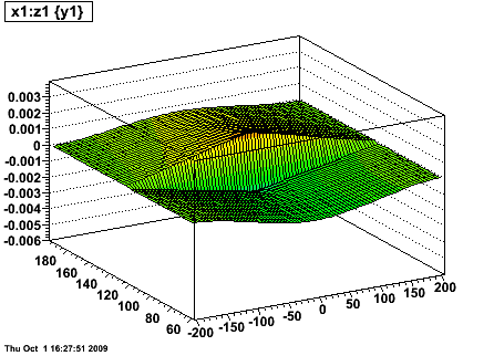
- Left: Surface plot showing the mean r-φ distortion we would get at the first iTPC pad row (radius = 55 cm) averaged over all active west-side z as a function of where the short is located ("ring of short") and how much external resistance is added.
- Right: Same but drawn as contours. The curve of interest to follow, that leads to <distortion>=0, is the one that starts near (ring,external resistance) = (110,0.0) and ends near (180,2.0), as indicated by the red markers. If the short is at ring 160.5, for example, then this curve indicates an external resistance of ~1.05 MΩ minimizes the distortions averaged over all active west-side z.
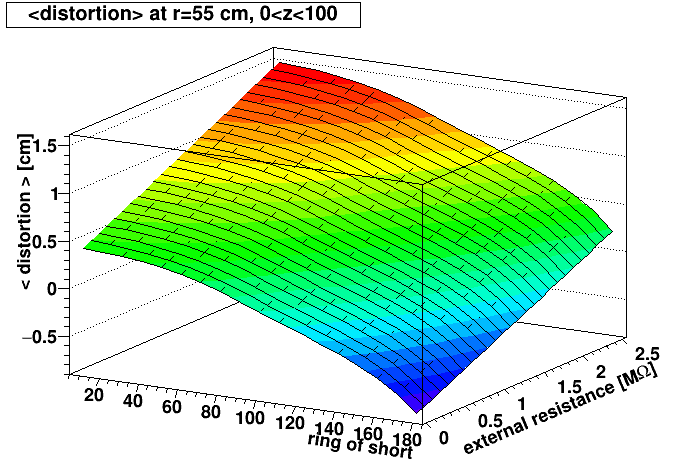
However, it may be more important to restrict the z range included in the distortion average, as most tracks of interest do not cross the inner pad rows at high z...
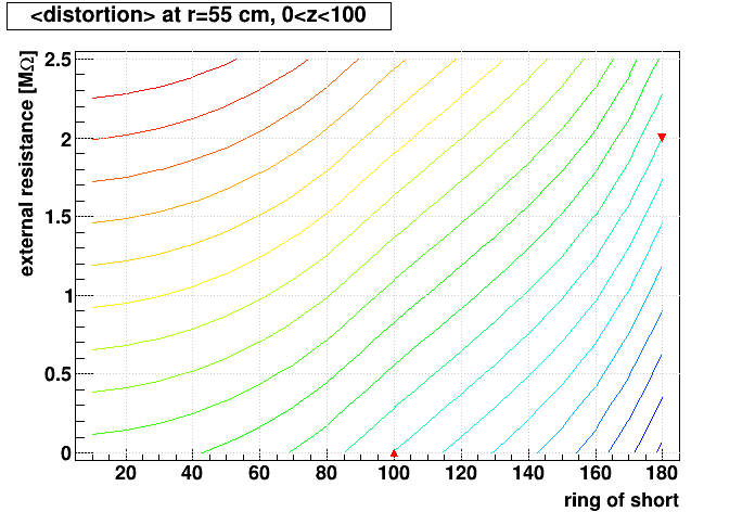
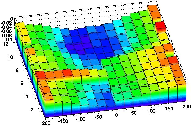
- Left: Similar surface plot, but restricting the average to 0 < z < 100 cm.
- Right: The curve of interest to follow in this contour plot, that leads to <distortion>=0, is the one that starts near (100,0.0) and ends near (180,2.0), as indicated by the red markers. If the short is at ring 160.5, then this curve indicates that an external resistance of ~1.25 MΩ minimizes the distortions averaged over 0 < z <100 cm.
Some additional observations:
- The curve of interest should always end close to (180.5,2.0), as that approaches the condition where the external resistance is no different than an internal resistance at the very end of the chain.
- The above is a simplification of what area should be integrated, as tracks with η ≠ 0 cross a variety of z at various radii, complicating the impact on their reconstruction. A track-by-track analysis of impact would be more meaningful, but a lot more work! The modeling shown here can serve as a rough guide to the best external resistance to use, but should not be taken as definitive for all physics.
- It is interesting to note that the model implies that a negative external resistance would help minimize the <distortion> when the short is closer to the central membrane (ring 0). A way to think of this is like having a short at both ends, such that the potentials are too high near the central membrane, and then too low near the endcap, so that the E field tilts one way in the region near the central membrane, isn't tilted at half the drift length, and then tilts the other way near the endcap, resulting in opposing distortions for electrons which drift the full length that serve to cancel each other. This could in principle be achieved by reducing the overall resistance of the Resistor box at the end of the Field Cage chain. The STAR TPC has (as of this documentation) had no persistent shorts near the central membrane that would warrant this approach.
-Gene
OFC West possible distortion
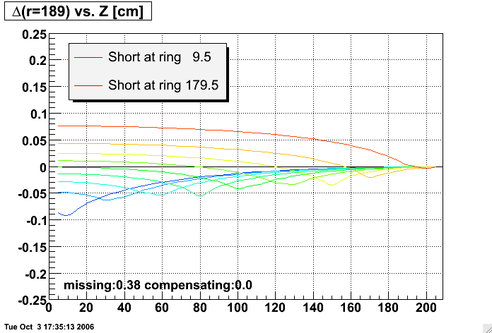
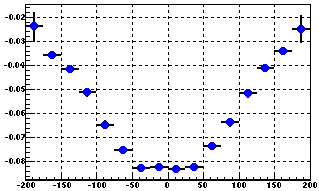
There remains a possible distortion due to a potential short in the OFC west as well. We see a bimodal pattern of 0 or 80 excess nanoAmps coming out of the OFC West field cage resistor chain (it has been there since the start of the 2005 run). That corresponds to a 0.38 MOhm short (420nA = 2 MOhms). The corresponding distortion depends on the location of the electrical short. The plot shown here is the distortion in azimuth (or rPhi) at the outermost TPC padrow near the sector boundaries (r=195 cm, the pads are closer to the OFC near the sector boundaries) due to such a short between different possible field cage rings:
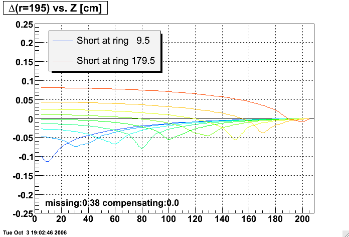
In terms of momentum distortion, a 1mm distortion at the outermost padrows would cause a sagitta bias of perhaps about 0.5mm for global tracks (and even less for primary tracks), corresponding to an error in pt in full field data of approximately 0.006 * pt [GeV/c] (or 0.6% per GeV/c of pt). This is certainly at the level where it is worthwhile to try to fix the distortion if we can figure out where the short is. It is also at the level where we should be able to see with the lasers perhaps to within 50cm where the short is.
Just as a further point of reference, the plot for radius = 189cm, corresponding to the radius of the outermost padrow in the middle of a sector (its furthest point from the OFC) can be found here.
This possible distortion remains uninvestigated at this time.
Gene Van Buren
gene@bnl.gov
Other FC short distortion measurements
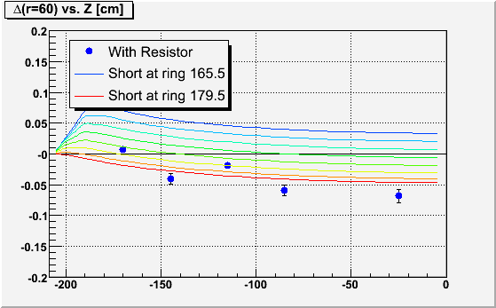
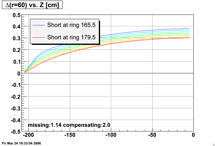
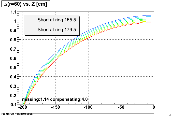
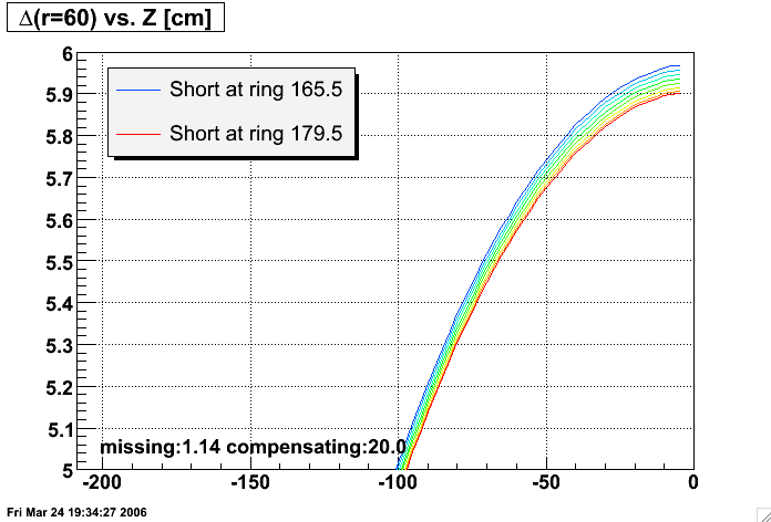
I considered the possibility that other measurements might help isolate the location of the short in the TPC. So, using the Modeled distortions, I modeled the effects of adding even more compensating resistance to the end of the IFC east resistor chain. Below are the results for shorts located at ring 165.5 (between rings 165 and 166), 167.5, 169.5, ..., 179.5 as indicated for the colored curves. All plots use a 1.0cm range on the vertical scale so that they can be easily compared. I had hoped that one resistance choice or another would cause more separation between the curves, giving better resolving power between different short locations. But this dependence is small, and actually seems to decrease a little with increased compensating resistance. Remember also that the last laser is at Z of about -173cm.Also perhaps worth noting is that the 1.0MOhm compensating resistor probably helps reduce the distortions even more than an exact 1.14MOhm would. The latter causes the distortions not to change between the short location and the central membrane, but the former actually causes the distortion to re-correct the damage done between the short location and the endcap!
| Compensating resistance [MOhms] |
Distortion on first padrow vs. Z |
|---|---|
| 0.0 |
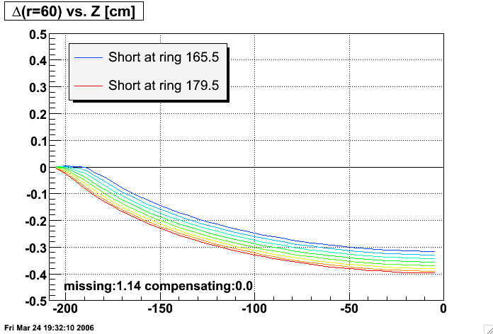 |
| 1.0 |
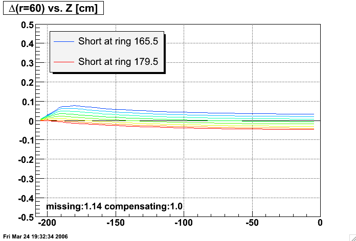 |
| 1.14 |
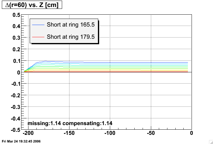 |
| 2.0 |
 |
| 4.0 |
 |
| 20.0 |
 |
Gene Van Buren
gene@bnl.gov
Observed laser distortions
First look
The first listed attached file was my initial look at distortions to laser tracks in the TPC (not that it is upside down from subsequent plots as I accidentally took the non-distorted minus the distorted here). These are radial tracks, and the plots are off the difference between run 7068057 (with excess current) and 7061100 (without excess current). Also, run 7068057 was taken with collisions ongoing, so there is some SpaceCharge effect as well (7061100 was taken without beam). I believe this explains the rotation of the tracks at low positive z (west side).
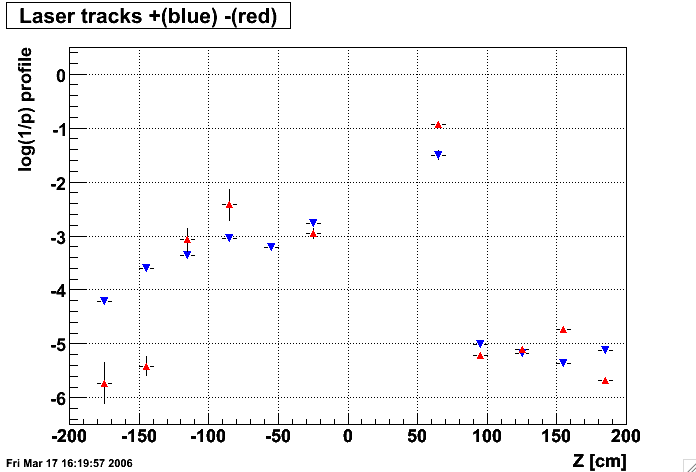
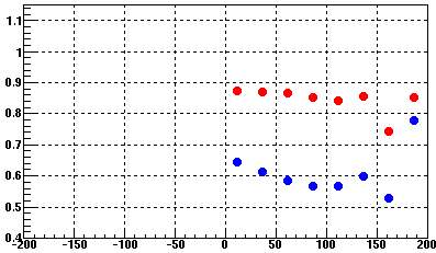
Second look: dedicated runs
On March 17, we took a couple laser runs without and with a compensating resistor to get the IFC east current at least approximately correct. I plotted 1/p of laser tracks and took the profile. Straight tracks give very low curvature = low 1/p. The distortion brings up the curvature, as can be seen in the IFC east without resistor. The same plot also shows large error bars for the negatively charged laser tracks because there aren't many: the curvature tends to bring them positive. The IFC west shows the appropriately low level without any distortion, but the timing on the west lasers was wrong, so they are not reconstructed where they are supposed to be in Z. I am uncertain whether this bears any relation to the odd behavior of the first laser on the west side (showing up here at Z of about +67cm). The IFC East plot for the no-compensating-resistor run also shows that 1/p begins to drop somewhere around Z of about -100cm. The short would be located where the largest slope occurs in this plot (because the distortion to tracks is an integral of the distortion in the field, and the short is where the field distortions are largest), but the data isn't strong enough to pin this down very well. The negative tracks indicate a short between the lasers at -145cm and -115cm. But the seemingly better quality positive tracks are less definitive on a location as the slope appears to get stronger at more negative Z, implying a short which is at Z beyond -170cm.
No compensating resistor (run 7076029):
With 1 MOhm compensating resistor (run 7076032), which brings IFC east current to correct value within ~20 nAmps, according to 10:27am 2006-03-17 entry in Electronic ShiftLog:

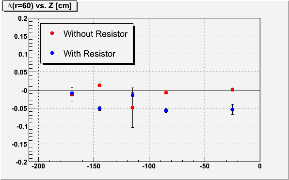
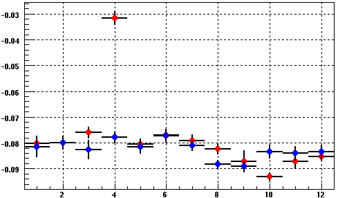
Again, I looked at the distortion as seen be comparing TPC hits from the distorted runs to those from an undistorted run as I did at the beginning of this page (but this time taking distorted minus undistorted). For the undistored, I again have only run 7061100 to work with as a reference. The plots for each Z are in the second listed attached file below, where the top 6 plots are for the no-compensating-resistor run (7076029), and the bottom 6 are the same ones with the resistor in. I also put on the plots the value of the difference from a simple fit (meant only to extract an approximate magnitude) at a radius of 60cm (approximately the first TPC pad row). Those values are also presented in the following plot as a function of Z, confirming the improvement of the distortion with the resistor in place.
These plots seem to point at a short which is occurring somewhere between the lasers at Z = -145 and -115cm.
Gene Van Buren
gene@bnl.gov
Resistor box at the end of the Field Cage chain
After ring 181, the potentials are determined by a box of resistors which sit outside the TPC. This is well documented, but at the time of this writing is not complete. This was particularly relevant during Run 9 when an electrical short developed inside the TPC between rings 181 and 182 of the outer field cage on the west end (OFCW). Shown here is a plot of the resistors:
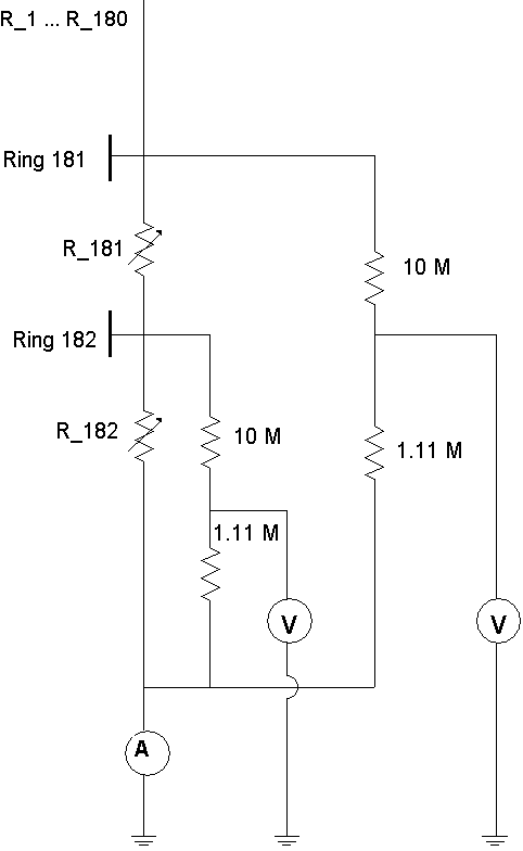
Note that the ammeter is essentially a short to ground, while the voltmeters are documented in the Keithley 2001 Manual to express over 10 GOhm of resistance (essentially infinite resistance). The latter only occurs when the input voltage is below 20 V. The voltages at rings 181 and 182 are above 20 V and below 200 V (though actually at negative voltage), so their voltage is scaled by the shown 1.11 and 10.0 MOhm resistors to be stepped down by a factor of x10. The readings are then multiplied by x10 before being recorded in the Slow Controls database.
After Run 9, this box was disconnected and resistances were measured for the OFCW portion. Because the resistors were not separated from each other, equivalent resistances were actually measured. In the below math, R182eq refers to the resistance measured across resistor R_182, while Rfull is the resistance measured between the input to the box from ring 181 to the output for the ammeter. R111 is the combined 10 + 1.11 MOhm pair.
double R111 = 10.0 + 1./(1./1.11 + 1./10000.)
11.11
double R182eq = 0.533 // measured
double Rfull = 2.31   // measured

double pa = R111 - Rfull
double pb = R111*(R111 - 2*Rfull)
double pc = (R182eq - Rfull)*R111*R111

double R181 = (-pb + sqrt(pb*pb - 4*pa*pc))/(2*pa)
2.3614
double R182 = 1./(1./R182eq - 1./R111 - 1./(R181+R111))
0.5841

double R182b = 1./(1./R182 + 1./R111)

double Vcm = 27960.
double Rtot = 364.44   // full chain
double Inorm = Vcm/Rtot
76.720
double V181_norm = Rfull * Inorm
177.22
double V182_norm = V181_norm * R182b/(R181 + R182b)
33.724

double Rshorted = 1./(1./R111 + 1./R182 + 1./R111)
0.5286
double Rmiss = Rfull - Rshorted
1.7814
double Ishorted = Vcm/(Rtot - Rmiss)
77.097
double V181_short = Rshorted * Ishorted
40.750
double Iexcess = Ishorted - Inorm
0.377
Note that many of these numbers would be different for the inner field cages.
External resistors to make up for missing resistance can also be added to the chain here.
GridLeak Studies
- Review of GridLeak at 2013-03-01 iTPC discussions
Floating Grid Wire Studies
Distortions in TPC data (track residuals) are seen in 2004-2006 data which are hypothesized to come from a floating Gating Grid wire. Notes from a meeting of TPC experts regarding the topic held in October 2006 can be found here.See PPT attachment for simulations of floating grid wires from Nikolai Smirnov which show that the data is consistent with two floating -190V wires in sector 8, and two floating -40V wires in sector 3 (all wires are at -115V when the grid is "open").
GridLeak Distortion Maps
Using the code in StMagUtilities, these are maps of the GridLeak distortion.
First, this is a basic plot of the distortion on a series of hits going straight up the middle of a sector (black: original hits; red: distorted hits). The vertical axis is distance from the center of the TPC (local Y) [cm], and the horizontal axis is distance from the line along the center of the sector (local X). Units are not shown on the horizontal axis because the magnitude of the distortion is dependence on the GridLeak ion charge density, which is variable.
The scale of the above plot is deceptive in not showing that there is some distortion in the radial direction as well as the r-phi direction. The next pair of plots show a map of the distortion [arb. units] in the direction orthogonal to padrows (left) and along the padrows (right) versus local Y and angle from the line going up the center of the sector (local φ) [degrees].
One can see that the distortion is on the order of x2 larger along the padrows than orthogonal to the padrows. Also, it is clear that there is a small variance in magnitude of the distortion across the face of the sectors.
The next plot shows the magnitude of the distortion [arb. units] along the padrow at the middle of the sectors vs. local Y [cm] and global Z [cm]. The distortion is largest near the central membrane (Z=0) and goes to zero at the endcaps (|Z| ≅ 205 cm), with a linear Z dependence in between, which flattens off at the central membrane and endcap due to boundary conditions that the perturbative potentials are due to charge in the volume and are constrained to zero at these surfaces.
GridLeak Simulations
Nikolai Smirnov & Alexei Lebedev:Data for STAR TPC supersector. 05.05.2005 07.11.2005 Jon Wirth, who build all sectors provide these data. Gated Grid Wires: 0.075mm Be Cu, Au plated, spacing 1mm Outer Sector 689 wires, Inner Sector 681 wires. Total 1370 wires per sector Cathode Grid Wires: 0.075mm Be Cu, Au plated, spacing 1mm Outer Sector 689 wires, Inner Sector 681 wires. Total 1370 wires per sector Anode Grid Wires:0.020mm W, Au plated, spacing 4mm Outer Sector 170 wires, Inner Sector 168 wires. Total 338 wires per sector Last Anode Wires: 0.125mm Be Cu, Au plated Outer Sector 2 wires, Inner Sector 2 wires. Total 4 wires per sector
We are most interested in the gap between Inner and Outer sector, where ion leak is important for space charge. On fig. 1 wires set is shown. The distance between inner and outer gating grid is 16.00 mm. When Grid Gate is closed, the border wires in Inner and Outer sectors have -40V, each next wire have -190V and after this pattern preserved in whole sector - see fig. 2. When gating grid is open, each wire in gating grid have the same potential -115V. Above grid plane we have a drift volume with E~134V/cm to move electrons from tracks to sectors and repulse ions to central membrane. Cathode plane has zero voltage, while anode wires for outer sector holds +1390V and for inner sector +1170V.

Fig. 1. Wire structure between Inner and Outer sector.

Fig.2 Voltages applied to Gating Grid with grid closed.
Another configurations of voltages on gating grid wires are presented on fig.3. All these voltages are possible by changing wire connections in gating grid driver. Garfield simulations should be performed for all to find a minimum ion leak.

Fig.3 Different voltages on closed gating grid (top: inverted, bottom: mixed).
This is a key for Nikolai's files: there are 4 sets of files in each set there is simulation for Gating Grid voltages on last wires. Additionally he artificially put a ground shield on the level of cathode plane and simulated collection for last-thick anode wire and also ground shield and last thin anode wire.
| Setups: | Standard | Inverted | Mixed | Ground Strip | Ground Strip and Wire |
|---|---|---|---|---|---|
| Equipotentials | PS |
PS |
PS |
PS |
PS |
| Electron paths | PS |
PS |
PS |
PS |
PS |
| Ion paths (inner sector) |
PS |
PS |
PS |
PS |
PS |
| Ion paths (outer sector) |
PS |
PS |
PS |
PS |
PS |
GridLeak: Gain Study
In February 2005, Blair took some special runs with altered TPC gains so we could study the effect on the GridLeak distortion. What is shown in the following plots is the distortion (represented by the profile of residuals at padrows 12 and 14, which amounts to 0.5 * [residual at padrow 12 + residual at padrow 14]) as a function of Z in the TPC. Black points are the distortions from sectors 7-24, and red are 1-6, which are the sectors where the TPC gain was reduced. I have chosen as labels "Norm", "Half", and "Low" for these three conditions of no gain change, half gain change on the inner pads only, and half gain change on both inner and outer.
First note: the ever-present problem that our model goes to zero distortion at the endcaps, while the measured distortions do not appear to do so (though the distortion curves should flatten out [as seen in the above plots] as a function of Z near the endcap and central membrane due to boundary conditions on the fields in the TPC).
Second note: I have not excluded sector 20 from these plots, which is partly to explain why the east half (z<0) has slightly less distortions than the west in these profile plots. In reality, east and west were about even for a normal run (distortions excluding sector 20).
Here is the z-phi plot for Low (it's almost difficult to see the distortion reduction in the z-phi (in "o'clock") plot for Half):
Third note: (though not too important for this study because we generally ignore east/west comparisons) the sectors between 1-6 o'clock already tend to show somewhat less distortion than the sectors at 7-12 o'clock, and because it is true on both halves of the TPC, it is more likely to be due SpaceCharge azimuthal anisotropy than asymmetries in the endplanes. Here are the distortions at |z|<50 for east (red) and west (blue) as a function of phi in "o'clock" where one can see the already present asymmetry, explaining why sectors 1-6 are already less distorted in the Norm run than sectors 7-12:
We have to normalize to sectors 7-12 to see the drop in distortions as it the runs are taken at different times when the luminosity of the machine, and therefore the distortion normalizations, are different. Here are the ratios from sectors 1-6 / sectors 7-12:

And the double ratios to see the drop in the Half and Low runs w.r.t. the Norm run:
These plots show ratios in the Z = 25-150cm range of about 0.86 and 0.59 respectively, or reductions of about 14% and 41% give or take a few percentage points. Data beyond 150cm tends to be poor and there's little reason to believe that the ratio really changes by much there. However, there does appear to be some shape to the data, which is not understood at this time.
Another way to calculate the difference in distortions is to take a linear fit to the slope of the distortions between z = 25-150cm. Those fit slopes are:
Low:
1-6: 0.000250 +/- 0.000019
7-12: 0.000420 +/- 0.000024
Half:
1-6: 0.000365 +/- 0.000023
7-12: 0.000433 +/- 0.000025
Norm:
1-6: 0.000401 +/- 0.000024
7-12: 0.000422 +/- 0.000023
Again, we need the ratio of ratios:
[Half(1-6)/Half(7-12)] / [(Norm(1-6)/Norm(7-12)] = 0.89+/-0.11 (12%)
[Low(1-6)/Low(7-12)] / [(Norm(1-6)/Norm(7-12)] = 0.63+/-0.08 (12%)
Inner reduction = (11 +/- 11)%
Outer reduction = (26 +/- 11)%
Total reduction = (37 +/- 8)%
These numbers are smaller than the reductions indicate by the above plot of double ratios of the distortions themselves. This likely reflects the errors in fitting the slopes. In that sense, the plot values may be more accurate. We need not worry in this study about getting the reduction numbers exact, but it is perhaps accurate enough to say that the inner sector gain drop reduces the distortion by about 13%, and the outer sector gain drop reduces it further by about 27% (about twice as much as the inner) from the original distortion. It is clear that both inner and outer TPC sectors contribute to the distortion, and that the outer TPC contributes significantly more to the distortion. If hardware improvements can only be implemented for either the inner or outer, then the outer is the optimal choice in this respect. It is not obvious offhand whether this is consistent with the GridLeak Simulations which we have done so far for these ion leaks.
Long term life time and future of the STAR TPC
In an effort to better understand the future of the TPC in the high luminosity regime, several meetings were held and efforts carried through.Present at the meeting(s) were: myself (Jerome Lauret), Alexei Lebedev, Yuri Fisyak, Jim Thomas, Howard Wiemann, Blair Stringfellow, Tonko Ljubicic, Gene van Buren, Nikolai Smirnof, Wayne Betts (If I forgot anyone, let me know).
It is noteworthy to mention that the TPC future was initially addressed at the Yale workshop in (Workshop on STAR Near Term Upgrades) where Gene van Buren gave a presentation on TPC - status of calibration, space charge studies, life time issues. While the summary was positive (new method for calibration etc...) the track density and appearance of new distorsions as the lumisoity ramped up remained a concern. As a reminder, we include here a graph of the initial Roser luminosity projection.
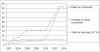
| 2002 | 2003 | 2004 | 2005 | 2006 | 2007 | 2008 | 2009 | 2010 | 2011 | 2012 | 2013 | 2014 | |
| Peak Au Luminosity | 4 | 12 | 16 | 24 | 32 | 32 | 32 | 32 | 32 | 48 | 65 | 83 | 83 |
| Average Au Store Luminosity | 1 | 3 | 4 | 6 | 8 | 8 | 8 | 8 | 16 | 32 | 55 | 80 | 80 |
| Total Au ions/ring [10^10] | 4 | 8 | 10 | 11 | 12 | 12 | 12 | 12 | 12 | 12 | 12 | 12 | 12 |
An update summary of the status of the TPC was given by Jim Thomas at our February
2005 collaboration meeting (A brief look at the future evolution of TPC
track distortions ; see attachement below) to adress ongoing GridLeak
issues. Slide 19 summary for teh future is added here:
Will the TPC Last Forever?
Probably of academic interest
Questions arose as per the liability of the detector itself i.e., aging issues (including shorts and side effects) were raised along with increasing concerns related to grid leak handling. Alexei Lebedev proposed a serie of hardware modification in May 2005 to account for those issues (see What we can do with TPC while FEE are in upgrade attachement).
Relevant to possible software and hardware solutions for the grid leak are GridLeak Simulations of the fields and particle paths in the region near the inner/outer TPC sector gap.
Extensive analysis are also available from the pages You do not have access to view this node and especially (for AuAu) this page QA: High Luminosity and the Future.
Anode wire aging
See the attached file: RD51-Note-2009-002.pdf
SpaceCharge studies
Studies of SpaceCharge in the TPC.
Potential distortions at projected luminosities for different species
Here I show the expected distortions in the STAR TPC as represented by the pointing error of tracks to the primary vertex (otherwise known as the DCA) due to experienced (star symbols) and projected luminosities (triangle and square symbols) at RHIC. One can think of these distortions as being caused by the accumulated ionization in the TPC due to charged particles traversing it from collisions (ignoring any background contributions), or the charge loading of the TPC.
These measurements and projections are current as of November 2008 with the exception of the pp500 (pp collisions at √s = 500 GeV) projections (open symbols) [1,2]. In 2005 the expectation was that RHIC II could achieve pp200 peak luminosities of 150 x 1030 cm-2sec-1 and pp500 peak luminosities of 750 x 1030 cm-2sec-1 [3]. Presently (2008), the pp200 peak luminosity estimate at RHIC II has dropped to 70 x 1030 cm-2sec-1, and this is what is used in my plot. I have found no current estimate for pp500. The 2005 estimate indicated a factor of x5 more peak luminosity from the 500 GeV running than 200 GeV; I do not know if that is still possible, but I have chosen to use only a factor of x2 (should be conservative, right?) in the plot shown here.
I have also had to estimate the conversion of luminosity into load in the TPC for pp500 as we have not yet run this way. We did run at √s of approximately 405 GeV in June 2005, which showed a 17% increase in load over pp200 per the same BBC coincidence rate [pp400 (2005)]. I have roughly estimate that this means approximately a 25% increase in TPC load going from pp200 to pp500, with no serious basis for doing so.
Finally, the documented projections show that RHIC II will achieve approximately a factor of x2.6 increase over RHIC I for both AuAu200 and pp200 [2]. I have taken the liberty to apply the same factor of x2.6 to CuCu200, dAu200, and pp500.
(Note: The pp data use a different horizontal axis which was adjusted to lie amidst the ion data for ease of comparison, not for any physically justified reasons.)
Of the data we've taken so far, AuAu collisions have presented the highest loading of the TPC. However, CuCu collisions have the potential to introduce the highest loading for ions, and the RHIC II projections lead to pointing errors close to 20 cm! Actually, SiSi may be even worse (if we ever choose to collide it), as the luminosity is expected to achieve a factor x4.2 higher than CuCu, while the load per collision may be in the 40-50% ballpark of CuCu [2,3].
Loading due to pp collisions at 200 GeV are generally similar to AuAu collisions at 200 GeV, but 500 GeV pp collisions will load the TPC much more severely. Even in RHIC I, we may have pointing errors between 5-10 cm using my conservative estimate of x2 for the luminosity increase over pp200. If the factor of x5 is indeed possible, then use of the TPC in pp500 at RHIC II seems inconceivable to me, as the simple math used here would completely break down (the first TPC padrows are at 60cm, while 2.5*25.1 cm is larger than that)**. Even with a factor of x2, things may be quite problematic for pp500 in RHIC II.
References:
Some additional discussions from 2005 regarding the TPC and increased luminosities are documented at Long term life time and future of the STAR TPC.
Note: This is an update of essentially the same plot shown in the 2007 DAQ1000 workshop (see page 27 of the S&C presentation).
** Actually, a rather major point: we never get full length tracks with DCAs to the primary vertex of more than a couple cm anyhow, due to the GridLeak distortion. These tracks get split and the DCAs go crazy at that point. Since GridLeak distortion corrections are only applied when SpaceCharge corrections are, an roughly appropriate SpaceCharge+GridLeak correction must be applied first to even find reasonably good tracks from which to determine the calibration.
SpaceCharge in dAu
In Run VIII, dAu data was acquired at high enough luminosities to worry about SpaceCharge (it was ignored previously in the Run III dAu data (2003)). Attached is initial work by Jim Thomas to determine the charge distribution in dAu.
TPC performance
Documentation on performance of the TPC
- Run 15 200 GeV p+Al Hit Errors
- Run 15 200 GeV p+Au Hit Errors
- Run 15 200 GeV p+p Hit Errors
- Run 14 (200 GeV Au+Au) TPC Hit Errors
- Run 14 (15 GeV Au+Au) TPC Hit Errors
- You do not have access to view this node (days 74-128) and You do not have access to view this node (pp510)
- Run 12 Cu+Au TPC Hit Errors
- You do not have access to view this node
- Run 12 pp510 hit errors
- You do not have access to view this node (You do not have access to view this node)
- You do not have access to view this node
- You do not have access to view this node
- You do not have access to view this node
- You do not have access to view this node, both pp500 and pp200, and re-calibrated You do not have access to view this node
- You do not have access to view this node (pp200, not certain it was Run 8 or an earlier dataset)
- You do not have access to view this node
TPC speed upgrade 2022
This page is setup to keep track of meetings documents for the task force work for thetpc speed upgrade for runs 23-25.
Status as of December 14 22,
Presentation from Tonko at collaboration meeting (pdf)
TPC meeting June 22
Update from Tonko on progress (pdf)
Meeting March 24
Discussion points send out ahead of meeting (Flemming) pdf
Progress slides - tonko pdf
minutes - Richard pdf
First meeting February 17
overview presentation and discussion (ppt)
minutes (pdf)
-
after meeting Jeff posted the projected resource needs for handling data to S&C (pptx)
Charge and Committee
TPX high rate test
- Discussion of test plans
- Discussion of test results
- Attached is a slide of the anode currents