I have previously noted instances of "stuck" 1-second RICH scaler readings in Run 8 data [1,Run 8 1-second scaler failures], and decided to work on a way to handle this. One option is to impose a cut during analyses. I have found a reasonably good cut to use for most of the pp data as:

19 < (zdcw+zdce)/zdcx < 28

Here, zdcw and zdce are the west and east ZDC singles rates, and zdcx is the ZDC coincidence rate. Using the 30-second scalers from the database, here is that quantity for the pp data:

 

Fig. 1: (zdcw+zdce)/zdcx versus run-9000000 for the Run 8pp data

 

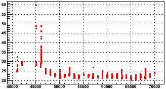
We see that for days before day 47, the cut won't work. So more investigation would be needed to fashion a cut for that data. Otherwise the 19-28 range is on the edge of what makes a good, simple cut because a doubling of any of the 3 scalers involved (zdce,zdcw,zdcx) almost always make a quantity which should fall in that range fall out (e.g. if the quantity should be 21, but one of the singles rate doubles, then you might get something like 31 instead). However, if zdcx and either, or both, of the singles scalers doubles, then it might get missed. Additionally, the zdce singles rate is typically about 80% of zdcw, so doubling zdce is less likely to get caught. And finally, the 1-second scalers in the data are likely to fluctuate a little more than the 30-second scalers used in the above plot, so there's a higher probability that normal events near the edge of the cut get excluded unintentionally.

It seems a better option to trap the doubling/tripling in the data itself. But how do you know when one of the scalers has got stuck? An obvious candidate for reference for the 1-second scalers is the 30-second scalers. Here's a plot of the ratio for zdcw from the pp data sample:

 

Fig. 2: (zdcw_1-sec / zdcw_30-sec) vs. time (in seconds, arbitrary offset - scale is x10³ in case you cannot read it)

 

 

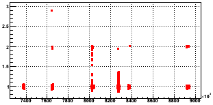
 There are obvious doubling and tripling of the zdcw 1-second rates, and there's some junk in the middle of the plot. I'll come back to the junk in a moment. While using the 30-second scalers for reference sounds good, there are some issues:

1. The code infrastructure will need some notable work to allow both the 1-second and 30-second scalers to be available.
2. The 30-second scalers do imply more database use, but this is a very minor issue for production and should be ignored.
3. There is some evidence that 30-second scalers show signs of getting stuck for an additional second or two also. I'll try to make that the subject of a different blog post.
4. At low scaler rates, it may not be easy to differentiate natural fluctuations from multiplications.

An alternative to using the 30-second scalers for reference is the value of the 1-second scalers from previous events. This has some drawbacks as well:

1. Some minor code change to store the value from the previous event.
2. The first event in the file will be unable to compare to anything.
3. Long time gaps between events within a single file (I've seen several minutes of gap) could be a concern.
4. Same as issue 4 for the 30-second reference.

A plot of zdcw 1-sec values versus the value from previous events looks similar to Fig. 2, so I won't re-show it. But because it is relatively easy to code this up, I went ahead and investigated what would make a good method to tag stuck (multiplied) 1-second scalers, and came up with the formula:

R_zdcw = zdcw / zdcw_previous

or R_zdce = zdce / zdce_previous  , etc. for all scalers

R' = abs(fmod(R+0.5,1.0)-0.5) < CutValue

This formula essentially gives how different a value is from an integer (the fmod over 1.0 lets me look for integrally multiplied values, while the +0.5 before and -0.5 after the fmod allow me to wrap-around the integers, it could be done other ways, no big deal). I propose the following cuts:

1. No cut for scaler < 100 Hz
2. No cut for R < 2.0 - CutValue
3. Otherwise, cut for R' < CutValue

This choice of cuts allows the scaler rates to fall naturally, but prevents upward jumps.

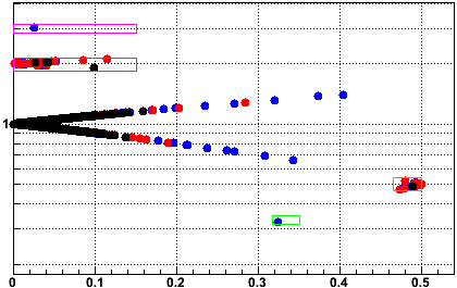
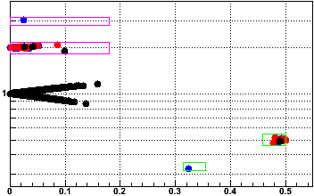
In Fig.3, I show in magenta boxes the exclusion regions in R vs. R' space of the data where I have used 0.15 for CutValue, and the data we wish to cut lies nicely inside those boxes (note that my definition of R' constrains the data to lie on a zig-zag path in this space). The green boxes are the inverse of the magneta boxes and are not cut; they highlight the "fall" back from a multiplied value down to a normal value (i.e. the scaler from the previous event was high). The colored data are zdcw(blue), zdce(red), and zdcx(black).

 

Fig. 3: R_zdcw vs. R'_zdcw

 

So this looks like a pretty reasonable cut technique, but one might ask about the data points in the middle of the plot. These correspond to the data in Fig. 2 which were strewn at values of R between 1.0 and 2.0. Looking more closely, they corresponded to three runs which were produced in this pp data sample which I used: 9056070, 9059058, and 9059067. The first and third of those are presently marked as questionable in the RunLog, so I'm not certain why they were produced. The second one was not marked as questionable. I believe all three should be marked questionable, and I discuss that below as an appendix to this post.

Anyhow, when I clean up the data by excluding those three runs, here are what Figs. 2 and 3 become:

 

Fig. 4: (zdcw_1-sec / zdcw_30-sec) vs. time (cleaned)

 

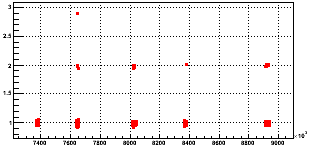
Fig. 5: R_zdcw vs. R'_zdcw (cleaned)

 

We can now see that there's a little more room than before to open the cuts, and here the boxes are made with CutValue = 0.18.

But what can be used to justify the value for the cut? I believe that answer is the fluctuation of the normal (non-multiplied) values. The zdc singles (blue,red) are buried under the zdc coincidence rate data points (black), which show the most variations event-to-event: as much as 0.16 (16%) in 50k events. Gaussian probabilities indicate that 1 event in 50k should happen at the 5.1σ level. This implies that σ is about 0.03 (I get a Gaussian fit σ value of 0.023 with some small tails, so this seems approximately reasonable). However, this is σ of f = x₁/x₂ (the ratio of two scaler readings), and we're actually interested in placing a cut on g = (x₁+x₂)/x₃ when a scaler gets stuck. So here's the math:

• σ(f)/f = √2 * σ(x)/x
• σ(g) = √(g²+2) * σ(x)/x = √((g²+2)/2) * σ(f)/f
• given g≅2 and f≅1, σ(g) ≅ √3 * σ(f) ≅ 0.05

If any of the scalers get stuck at a rate of once per 5k events for any given scaler (the highest rate I have seen in the sample), then we might expect about 10k stuck values of any scaler in 50M total events. To probabilistically avoid missing those, we need to go to about 4σ, or a CutValue of about 0.20.

A detail worth some consideration is that the first event in a file will not be tag-able. For the pp data from Run 8, the average file has about 10³ events, so probabilistically 10 out of 10k stuck values will be the first event in a file. We correct SpaceCharge using zdce+zdcw, so I expect about 2*10 = 20 files out of the full production will be impacted. It may be possible to simply discard these files, or this may even be at a level sufficiently low not to impact anyone's physics (20 events out of tens of millions). One might expect that long time gaps between events within files might pose problems too (I have seen gaps of several minutes in the past within a file), but this was certainly not an issue for the pp data from Run 8, where the lifetime of the beam was impressively long (τ ≅ 10-15 hours), so a 10 minute time gap would naturally lead to only a very small change in rates.

The last question is what to do with tagged instances of high scalers. The simplest answer is to use instead the reference value to which it was compared instead and keep using it as the "previous" value until a good new one comes along.

I have implemented the necessary code in StDetectorDbMaker, and put the CutValue into the database. Since it only needs to be defined once per species' dataset (if that), I have put it in the ZeroField column of the SpaceCharge table (this column has never been used, and SpaceCharge is the primary consumer of the RICH scaler data anyhow).

 

---

Appendix:

 

(NOTE: the follow-up below this post has an explanation for these runs)

As an example of what's bad about these particular runs mentioned earlier (9056070, 9059058, and 9059067), here is one of the single scalers from fill 9966, which includes the two runs I have from day 59 marked as red data points:

 

Fig. A1: Fill 9966 zdcw_30-sec vs. time (in seconds, arbitrary offset - scale is x10³ in case you cannot read it)

 

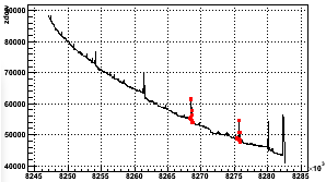
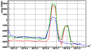
All the singles scalers look almost exactly like that for fill 9966. As I have no idea what is causing those "blips" in the scalers, I wouldn't trust data acquired during that time very much and the data should be marked questionable. Interestingly, the blips seem to occur with a regular interval of about 7.2 x 10³ seconds and have very similar structure as shown in this overlaid plot (Fig. A2) of the 4 peaks at about 8254(blue), 8261(green), 8269(red), and 8276(black) (x10³) from Fig. A1. For each curve, I simply subtracted off a background which scaled down by a factor of 0.88 which each successive peak. So the offset for the vertical axis is a bit arbitrary, but the impressive thing is that the last 3 of these peaks show identical absolute magnitude and double-hump structure. Something odd was occurring at RHIC with a regularity of almost 2 hours! It's a mystery...

 

Fig. A2: Fill 9966 zdcw_30-sec peaks overlaid

 

The conclusion is that there are questionable runs which will need to be found. It will be easier to scour the 30-second scalers from the DB for anomalies like this, but it is more difficult to see these anomalies in the 30-second scalers as they get dampened by the longer time average. This much will require further investigation.

 

FOLLOW-UP: The blips (for all three of the mentioned runs) are explainable as times when the CNI polarimeter measurements occurred (every approximately 2 hours), disrupting the beam to some extent. I still believe all of these runs should be marked questionable.

 

---

-Gene