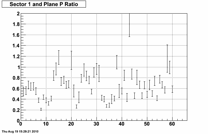
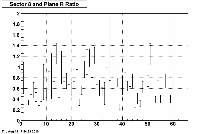
2009 EEMC 200 GeV MIP calibration Preliminary Pre/Post Fits
Introduction
After completing the preliminary analysis of SMD gains using slopes, I moved on to get preliminary fits for the two preshower layers (P and Q) and the postshower layer (R).
In the code now, the fitting was done with a non-compiled macro for the pre and post shower layers. However, the smd uses a compiled class called SmdGains. I wanted to change the fitting to use something compiled as well. I've noticed Root will let you do crazy things with non-compiled code. Also, the fitting should be faster this way. Another bonus is that I included the fast and slow simulators to consistently use the sampling fraction and MIP dE/dx found there. I also added some functionality for getting preliminary gains from slopes, though I did not extensively test or use it at this time.
The requirements imposed when looking for the MIP signal then were:
- MIP signal in the shower max with 7 empty strips on either side
- Energy deposit in the towers (using ideal gains) consistent with MIP within a window of 1/2 to 2 times the expected MIP energy.
no requirements are made on the preshower or postshower layers.
The distributions are fit with a Landau function and a constant offset term. This produced overall good fit quality while not introducing too many fit parameters. The fit range is taken as max(1.5,Mean-60) to min(150,Mean+100). Visual inspection showed that the histogram mean was often close to the peak or most probable value. This might need to be changed when final gains are fit. The fit range is denoted by the green lines on the plots.
Results
PDF files with the fits for each tile and layer are attached in the zip file. You may need to zoom in to see the titles. The pattern is left->right is subsector A->E and top->bottom is eta bin 1->12. The gain file and mask files attached were also used. I inspected the mask file and verified the entries by eye. If the distribution looked fine but fit failed, I removed the mask and used the gain from a neighboring subsector. I did notice that Sector 5 distributions looked quite funny for all the layers. Many of these distributions are masked out.
Also attached is a file called compareAllLayers.pdf that shows the ratio of the gains here to the final 2006 gains. Overall this ratio seems low.
Gain and mask files are also attached.
Next Step
My next step is to feed these prelimary gains and the mask file back to the calibration. Then I can re-fit these layers and the towers using the "constrain all but this layer" approach to get gains. One final iteration might be needed after that.
Update 23 August
After I tried fitting the towers the first time the gains were coming out very low. I realized that when I updated the code to use the sampling fraction and dEdx from the simulator that this would cause an inconsistency with the currently loaded ideal gains, which assumed a 5% sampling fraction. I re-ran the code with the old values and re-fit for preliminary gains. I see to have a few less tiles masked out this time (~11). The inclusive distributions with slope fits (not used at this time) are also included in the zip file this time.
Update 24 August
This one is important! To get the gain we use the expected energy deposited by a MIP. These values are the means and not the most probable values. In the past, this was fixed after the fact by using a factor of 1.46 from simulations to go from MPV->mean. Root's TF1 class will calculate the moments of your functions. I'm having it calculate the mean over the fit range and using that (not surprisingly it's close to 1.46 times the MPV). I'm refitting all the layers and then will go back and try to do a preliminary fit of the towers again. Towers end up looking really Gaussian (go go central limit theorom) and this is not so important for them.


- aliceb's blog
- Login or register to post comments
