- drach09's home page
- Posts
- 2022
- 2020
- June (1)
- 2019
- 2018
- 2017
- 2016
- 2015
- 2014
- December (13)
- November (2)
- October (5)
- September (2)
- August (8)
- July (9)
- June (7)
- May (5)
- April (4)
- March (4)
- February (1)
- January (2)
- 2013
- December (2)
- November (8)
- October (5)
- September (12)
- August (5)
- July (2)
- June (3)
- May (4)
- April (8)
- March (10)
- February (9)
- January (11)
- 2012
- 2011
- October (1)
- My blog
- Post new blog entry
- All blogs
2006 EEMC Neutral Pions: Background Correction (Alternative Method v3.0)
(January 18, 2012) NOTE: From this update until my December 31 update I incorrectly calculated the background-asymmetry systematic. I have subsequently changed my methodology. Instead of taking the largest asymmetry from among the bins, I take the largest average of the two bins surrounding the pion peak (turns out to be the yellow beam). This is ~2%. The sizes of the resulting systematics are quite comparable to what has been reported.
I have now ported everything over to run Steve's code, again. Ultimately, I would like to check Steve's direct method of background subtraction. However, I still lack a few tools (or perhaps the just knowledge to use them); and time grows ever short. This update, I report the asymmetries from Steve's runlist with the full slate of systematic errors (pending further suggestions). Namely, I include systematics for
- Varying the background asymmetry
- Propogating errors from the mass fit parameters and the residuals for those fits
- Calculating the asymmetries with a different background fitting method
- Calculating the asymmetries using a different mass window
Unless I receive further suggestions or "bolts from the blue" I will assume the systematics are satisfactorily covered.
There are additional runs from Steve's list which I may integrate. Steve has restricted himself to runs including the TPC and luminosity information. Since the cross-ratio cancels out luminosity (and the "traditional method" allows one to factor luminosity asymmetries into a constant term) it seems like we could use these additional runs. It may also be possible to utilize the runs absent the TPC, however, this probably merits further discussion.
Signal Fraction
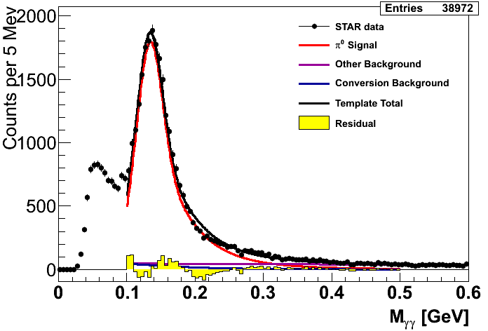
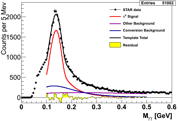
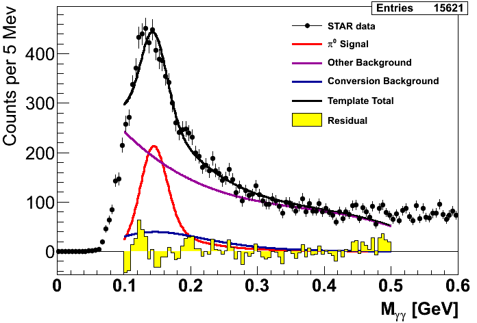
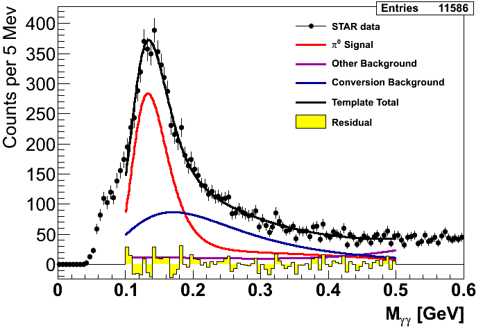
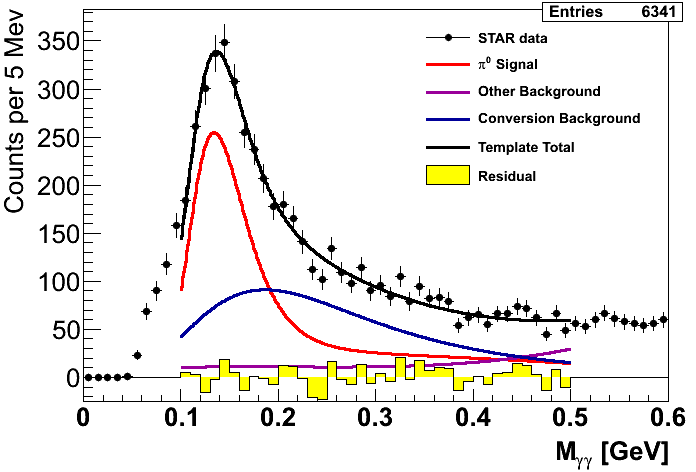
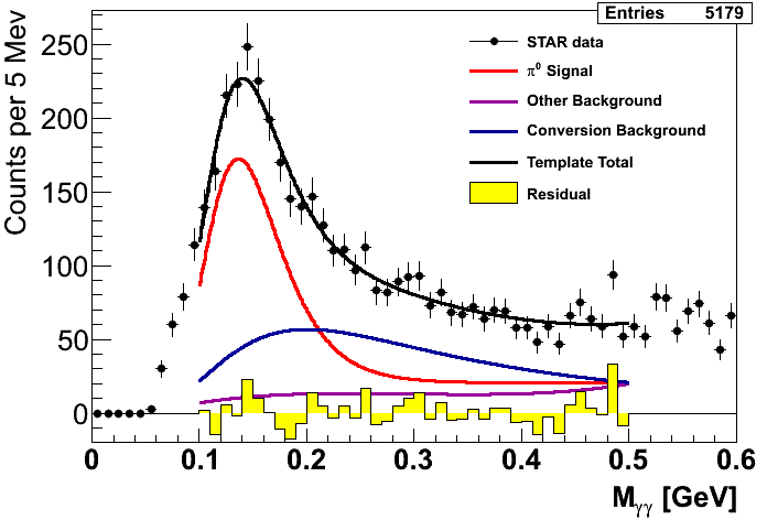
Again, I calculate the signal fractions utilizing Steve's method of applying the template fits to the data summed over φ and spin state. The "signal" mass window is taken as 0.1 < mγγ < 0.2 GeV/c2. The errors (propagated errors and residuals) from this fit are applied as statistical uncertainties and also factored into the systematic errors.
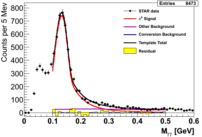
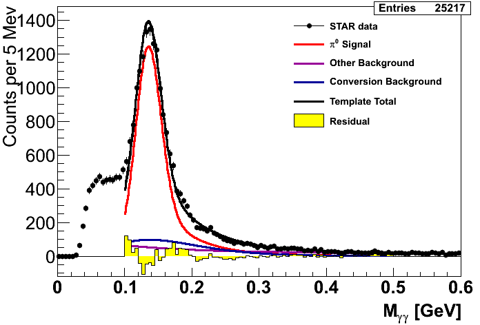
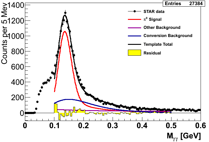
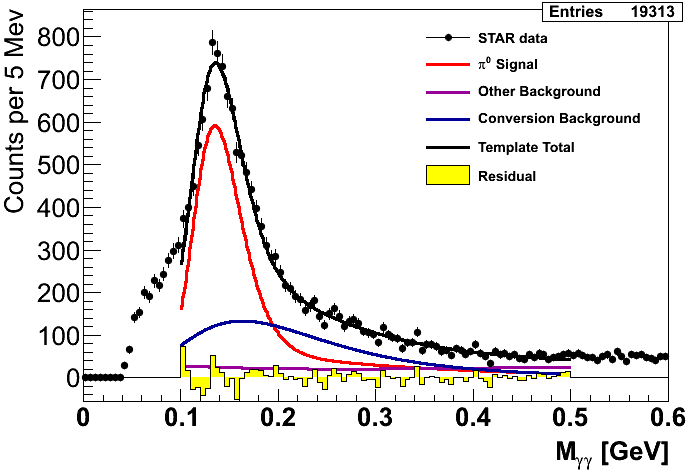
Figure 1
| xF Bin 1 | xF Bin 2 | xF Bin 3 |
|---|---|---|
 |
 |
 |
| pT Bin 1 | pT Bin 2 | pT Bin 3 |
 |
 |
|
| pT Bin 4 | pT Bin 5 | pT Bin 6 |
 |
 |
 |
| pT Bin 7 | pT Bin 8 | pT Bin 9 |
 |
 |
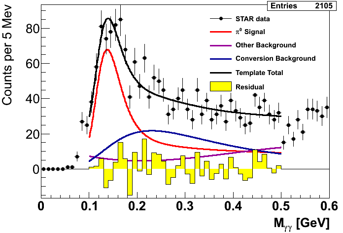 |
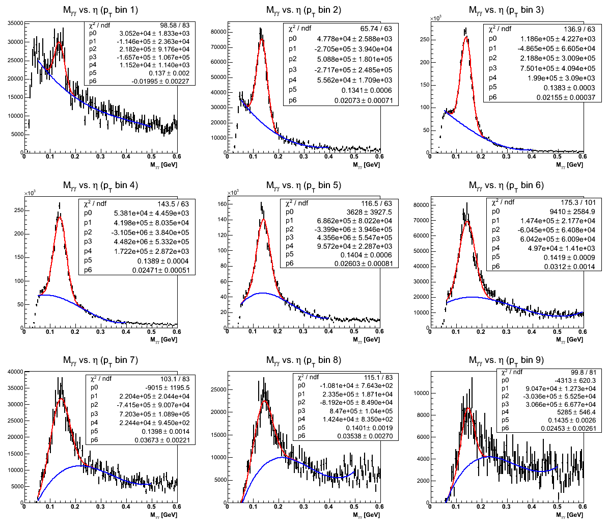
Figure 1 shows the mass fits from Steve's method. The first pT bin is left empty as our Monte Carlo match to the data is unacceptable. Recall that the xF bins integrate pT bins 2-9 and are thus unaffected by this disagreement with the first pT bin. One can immediately see that in the highest-xF bin the fit is not quite ideal. It may be possible to improve this fit, so I will revisit this issue in the future. One also sees that in several bins there are low-mass features which the fits do not seem to match. Our guess is this is related to imperfect GEANT modeling of material in front of the EEMC. It is, thus, important to understand our sensitivity to uncertainty in the background under the peak. To this end I investigate two studies: varying the background fitting methodology and varying the mass window.
Again, I employ a Gaussian-signal+polynomial-background function (3rd order polynomial) as an alternative way to model the background. I have checked that it makes no difference to use the measured or the upper-limit background asymmetry in this procedure. For these figures I have used the upper-limit, but from here on out I will probably use the measured value. The difference between the calculation utilizing the fits from Fig. 1 and the alternative fits shown in Fig. 2 determines the signal fraction systematic uncertainty.
Figure 2
|
xF Bins |
|---|
|
|
|
pT Bins |
|
|
There is no physics-process-driven motivation for the fits in Fig. 2, and in that sense our methodology from Fig. 1 is more sound. Thus, our central values come from our Monte Carlo methodology. However, given the inconsistencies of the Monte Carlo in modeling the low-mass features of Fig. 1, I argue it is reasonable to turn to a data-driven methodology to estimate our sensitivity to variations in the low-mass background under the signal peak. This methodology is not universally accepted as appropriate, however, and some discussions remain before I am confident to proclaim these results ready for broader consumption or "preliminary result" status.
One other note worth mentioning is my handling of the first pT bin. As you can see, the peak is quite small relative to the background. We will ultimately exclude this bin and perhaps others from our publication, however, I have kept it in the analysis for the time being. To handle the systematics for this bin I apply a second data-driven fit using a 2nd-order polynomial for the background. The signal fractions for this bin, thus, are calculated entirely from integrating the data-driven fits.
The final systematic I have checked is to vary the mass window. I do this by recalculating the asymmetries by integrating the mass from 0.12 < mγγ < 0.18 GeV/c2. For this I also recalculate the signal fractions in the peak for the new mass window. The difference between the asymmetries calculated from the standard window and the new window set the systematic uncertainty. In most cases, this actually counts as the leading systematic uncertainty.
Asymmetries
Here, I post the current status of the asymmetry calculations.
Figure 3
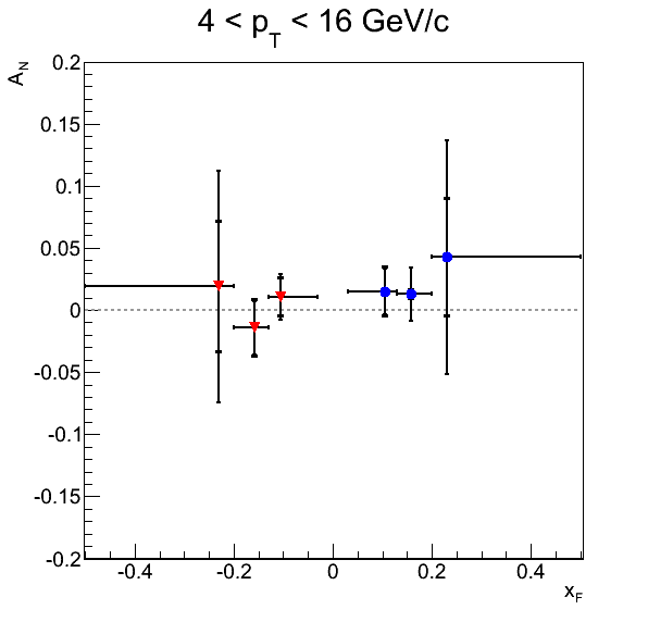
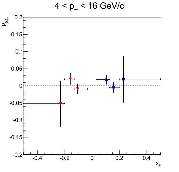
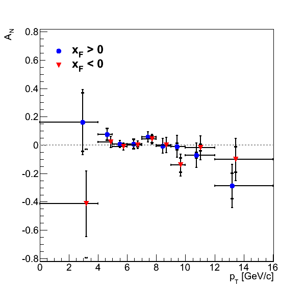
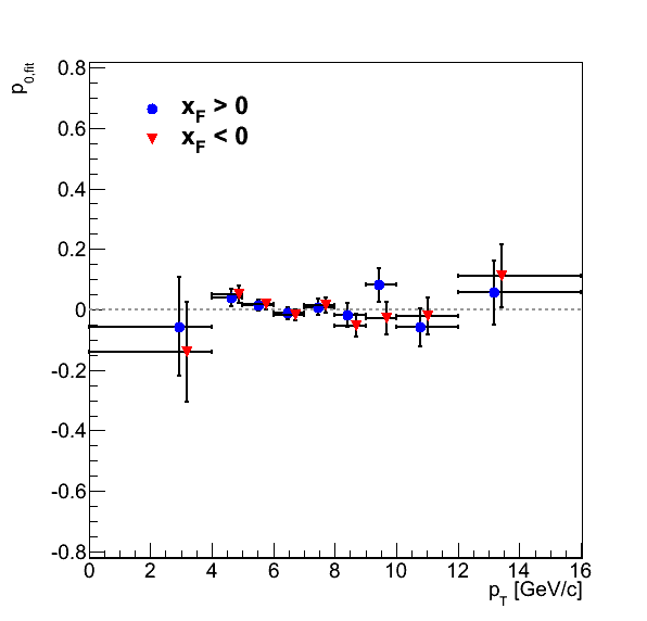
Figure 2 shows the background-corrected pion asymmetries as well as the p0's for the φS fits. Normal error bars are statistical errors, while bracket-style error bars are systematic. For clarity I have posted data tables below. Of twenty-four total bins, five show systematic errors greater than the statistical uncertainties. Three of these bins (xF > 0: xF Bin 1, pT Bin 4; xF < 0: xF Bin 2) are dominated by the mass-window systematic. One bin (xF > 0: pT Bin 2) is dominated by the signal-fraction systematic using the polynomial fit method. Finally, pT Bin 1 for xF < 0 is dominated by the systematic errors propagated through fit parameters. Of course, this bin does not utilize the Monte Carlo fitting and will not be included in the publication. The large systematic appears to be driven by the large raw asymmetry (probably a statistical fluctuation) and the very small signal fraction extracted by the functional fit. Given that in only four bins is the signal-fraction systematic the largest, it seems at this stage our methodology is not terribly sensitive to the alternative fitting method. However, in most cases (18 bins) our leading systematic is the mass window. This suggests to me that we are still sensitive to underlying backgrounds. However, in most cases, we tend not to be sensitve above the level of our statistical uncertainties. It will be interesting to see if this remains true after integrating a few more runs.
Table 1: xF > 0
| AN | δAN Stat | δAN Total Syst | δAN B.g. Asym Syst | δAN Sig. Fit Param. Syst | δAN Sig. Frac. Syst | δAN Mass Window Syst | |
|---|---|---|---|---|---|---|---|
| xF Bin 1 | 0.014952 | 0.018486 | 0.020128 | 3.55421e-05 | 0.000357631 | 0.0076375 | 0.0186196 |
| xF Bin 2 | 0.012732 | 0.021515 | 0.004268 | 6.78711e-05 | 0.000494245 | 0.00408929 | 0.00111751 |
| xF Bin 3 | 0.042639 | 0.094089 | 0.047778 | 0.0003745 | 0.00669747 | 0.0211153 | 0.0423305 |
| pT Bin 1 | 0.161096 | 0.230120 | 0.208512 | 0.00263509 | 0.150673 | 0.0103346 | 0.143739 |
| pT Bin 2 | 0.076947 | 0.040340 | 0.043262 | 9.58145e-06 | 0.00109368 | 0.043065 | 0.00398113 |
| pT Bin 3 | 0.006119 | 0.025169 | 0.001880 | 0.000110819 | 0.000377792 | 0.00115395 | 0.00143058 |
| pT Bin 4 | 0.007489 | 0.027339 | 0.036842 | 9.87453e-05 | 0.000422925 | 0.000816747 | 0.0368304 |
| pT Bin 5 | 0.056686 | 0.035909 | 0.013119 | 0.000172764 | 0.00205633 | 0.00573741 | 0.0116162 |
| pT Bin 6 | -0.005457 | 0.053214 | 0.002921 | 8.44989e-06 | 0.000173617 | 0.000554019 | 0.00286222 |
| pT Bin 7 | -0.010149 | 0.077106 | 0.025297 | 2.88347e-05 | 0.000481477 | 0.0002319 | 0.0252914 |
| pT Bin 8 | -0.071859 | 0.085738 | 0.023012 | 5.3972e-05 | 0.00446704 | 0.0168814 | 0.014987 |
| pT Bin 9 | -0.288682 | 0.152318 | 0.090637 | 0.000212938 | 0.0211231 | 0.0551557 | 0.0687508 |
Table 2: xF < 0
| AN | δAN Stat | δAN Total Syst | δAN B.g. Asym Syst | δAN Sig. Fit Param. Syst | δAN Sig. Frac. Syst | δAN Mass Window Syst | |
|---|---|---|---|---|---|---|---|
| xF Bin 1 | 0.010541 | 0.018254 | 0.016146 | 1.80583e-06 | 0.00025903 | 0.00529453 | 0.0152514 |
| xF Bin 2 | -0.014269 | 0.021259 | 0.023044 | 7.3947e-06 | 0.000474286 | 0.00376293 | 0.0227296 |
| xF Bin 3 | 0.018926 | 0.092948 | 0.052955 | 0.000137871 | 0.00306197 | 0.00940055 | 0.0520234 |
| pT Bin 1 | -0.413140 | 0.231640 | 0.384711 | 0.00883788 | 0.382943 | 0.0306607 | 0.0183986 |
| pT Bin 2 | 0.020784 | 0.039833 | 0.012158 | 2.06567e-06 | 0.000306126 | 0.011413 | 0.00417843 |
| pT Bin 3 | -0.010657 | 0.024855 | 0.008364 | 0.000559459 | 0.000506685 | 0.00447443 | 0.00702609 |
| pT Bin 4 | 0.000210 | 0.027073 | 0.014582 | 0.000250585 | 6.22621e-05 | 0.00227701 | 0.0144006 |
| pT Bin 5 | 0.041416 | 0.035436 | 0.026730 | 1.54264e-05 | 0.00151246 | 0.00831426 | 0.0253592 |
| pT Bin 6 | -0.000335 | 0.052602 | 0.011482 | 1.41811e-05 | 2.80153e-05 | 4.72227e-06 | 0.0114821 |
| pT Bin 7 | -0.141673 | 0.076293 | 0.053644 | 3.28869e-05 | 0.00743854 | 0.000262558 | 0.0531248 |
| pT Bin 8 | -0.019415 | 0.084925 | 0.025163 | 0.000778979 | 0.00115873 | 0.0144604 | 0.0205461 |
| pT Bin 9 | -0.102171 | 0.150345 | 0.091771 | 0.000184618 | 0.00742627 | 0.0172674 | 0.089825 |
- drach09's blog
- Login or register to post comments


