Luminosity Matching

Our embedding procedure simulates jet events with PYTHIA which are then embedded in zerobias data. It is important to select a subset of zerobias files which sample the characteristic luminosity of the set of runs from which we analyze jets.

Figure 1

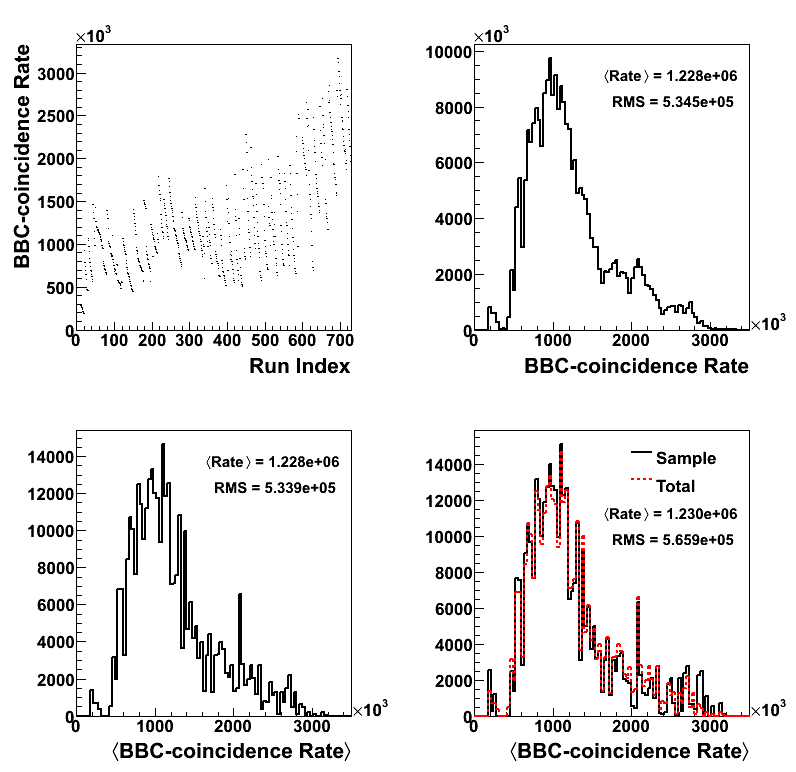
In the upper right-hand panel of Fig. 1 I plot the BBC-coincidence rate as a function of run from the values obtained in the jet trees. One can clearly see the fill structure, as the coincidence rate declines with the runs within a fill. The coincidence rate of all events is binned in the upper left-hand panel. Displayed are the mean rate and standard deviation of the distribution.

The idea is to select from the set of zerobias runs in such a way that the events add up to reflect the shape of the total run list. In the bottom left-hand panel I plot the average rate for each run, weighted by the number of events in the run, again taking the values from the jet trees. The histogram is then normalized so that the integral is 350,000 (the projected number of embedding events). I then loop over the zerobias run list and select runs until the event totals for the corresponding coincidence rate reach the values reflected in the bottom left-hand histogram. The result is shown in the bottom right-hand panel of Fig. 1. In black is the resulting distribution from the zerobias files. In red is shown the distribution from the jet trees for comparison. The resulting mean and standard deviation are quite close to that of the full dataset. The general shape is also quite close to what we observe in the trees. A text file with the desired zerobias DAQ files is attached at the bottom of the page.

It is, then, necessary to choose the event numbers for each partonic p_T bin for each run. For each run, the event numbers for each partonic p_T bin are chosen by scaling the event total for the run by the fraction of total events which the bin represents. The event number lists are attached at the bottom of the page.

Partonic Scaling

In addition to matching the luminosity of the Run-11, it is important to ensure that the partonic p_T bins are appropriately scaled for a smooth partoinc p_T-distribution. Here, I have implemented a scale of the form f×σ_part/N_evt, where N_evt is the number of events PYTHIA generates for the p_T bin, σ_part is the average partonic cross section from the PYTHIA log, and f is a fudge-factor determined by fitting functions to the partonic p_T distribution. In this case, I use a polynomial distribution below p_T = 35 GeV/c and otherwise an exponential. The resulting fudge-factors are

const float fudge[] = {
    1.000000000,
    1.470915199,
    1.680658589,
    1.733102356,
    1.737224156,
    1.759743735,
    1.763468949,
    1.748911256,
    1.759581377,
    1.758756016,
    1.829962421,
    1.780396640,
    1.749266858,
    1.739892600,
    1.724057566
};

Figure 2

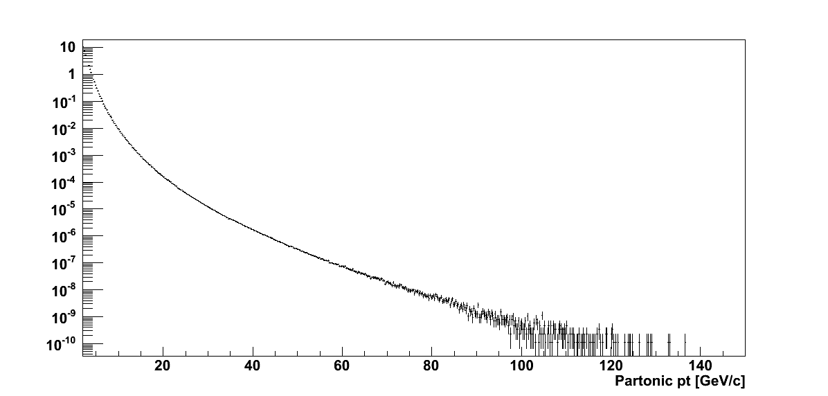
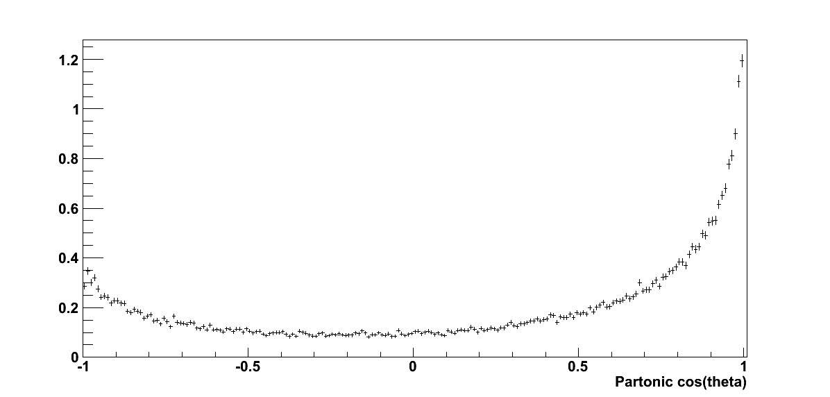
In Fig. 2 I plot resulting distributions for the partonic p_T and cos(θ). The resulting distributions are quite smooth over quite a range of partonic p_T. Additionally, the cos(θ) distribution appears smooth.

Vertex Weighting

For the vertex weighting I simply ask if a particular trigger fired. Thus, VPDMB is take-all. For the jet triggers, I apply the weight for the highest available trigger.

Figure 3

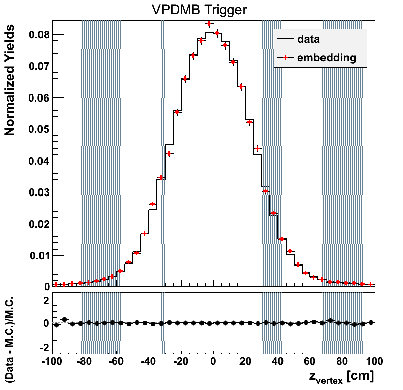
Figure 4

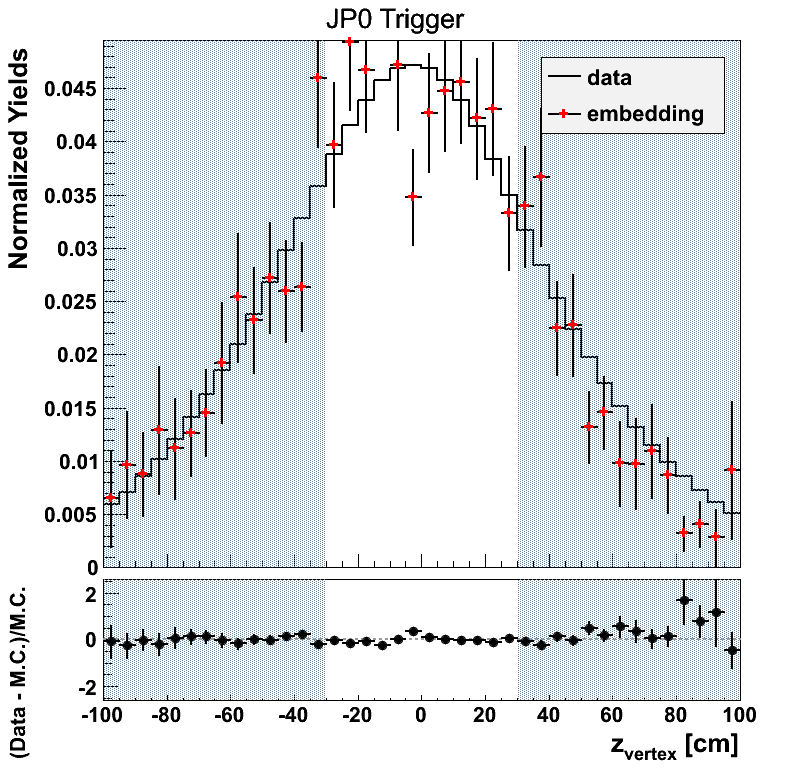
Figure 5

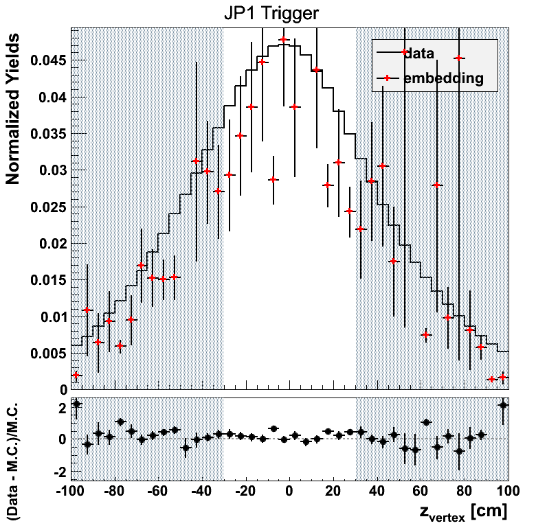
Figure 6

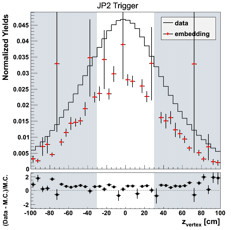
The weighting for JP2 appears off by a constant scale factor. This appears to be the result of a few low-statistics bins which throw off the normalization. In general the weighting should work for the sake of comparing embedding to data.

Trigger Definition

The way I define my data triggers is not workable in the embedding. For example, every time JP2 "should fire," JP1 will register "should fire." Since in the data I define JP2 "(JP2||AJP)&&!JP1&&!JP0&&!VPDMB" this formulation will never lead to a JP2 trigger in embedding. For a first glance, I will use a different definition, as follows:

VPDMB = pT < 16.3 GeV/c
JP0 = shouldFire(JP0) && pT > 7.1 GeV/c && ( (!shouldFire(JP1)||(pT < 9.9 GeV/c) ) && ( (!shouldFire(JP2)&&!shouldFire(AJP)) || (pT < 16.3 GeV/c) )
JP1 = shouldFire(JP1) && pT > 9.9 GeV/c && ( (!shouldFire(JP2)&&!shouldFire(AJP)) || (pT < 16.3 GeV/c) )
JP2 = shouldFire(JP2)||shouldFire(AJP) && pT > 16.3 GeV/c

I believe this formulation follows quite closely with what Pibero used for JP1 and L2JetHigh for the 2009 analysis.

η-φ Comparison

Figure 7

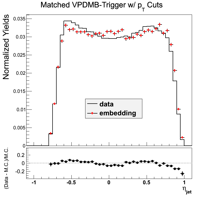
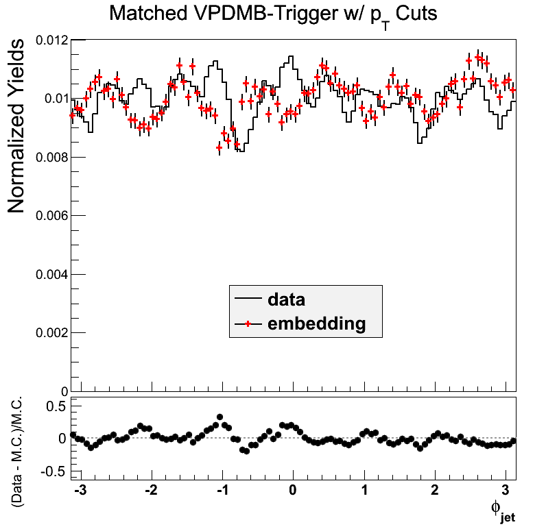
VPDMB is take-all between 5 and 16.3 GeV/c. The agreement in eta is not so bad. The agreement in phi is not great. There may be a hint of jet-patch structure visible which may be part of the issue.

Figure 8

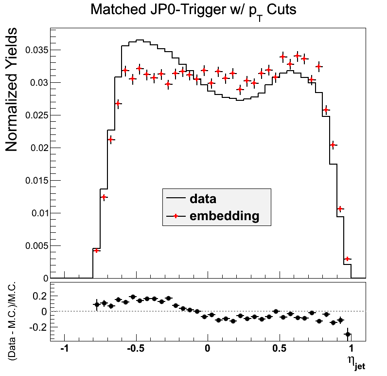
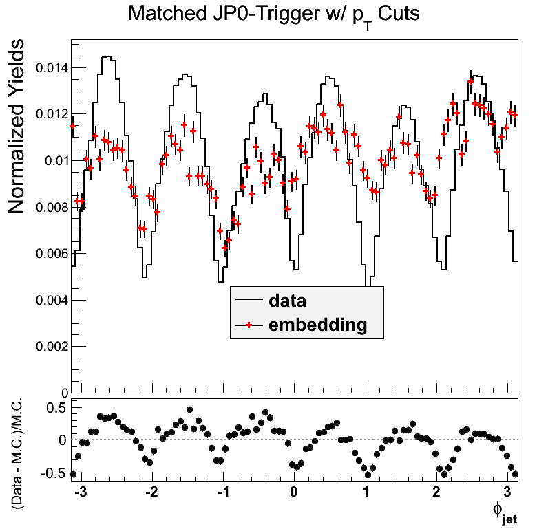
The agreement in JP0 is a bit off near -0.5. In phi the peak-to-valley ratio is quite a bit smaller in the embedding. My first reaction would be to attribute this to AJP possibly leaking into JP0.

Figure 9

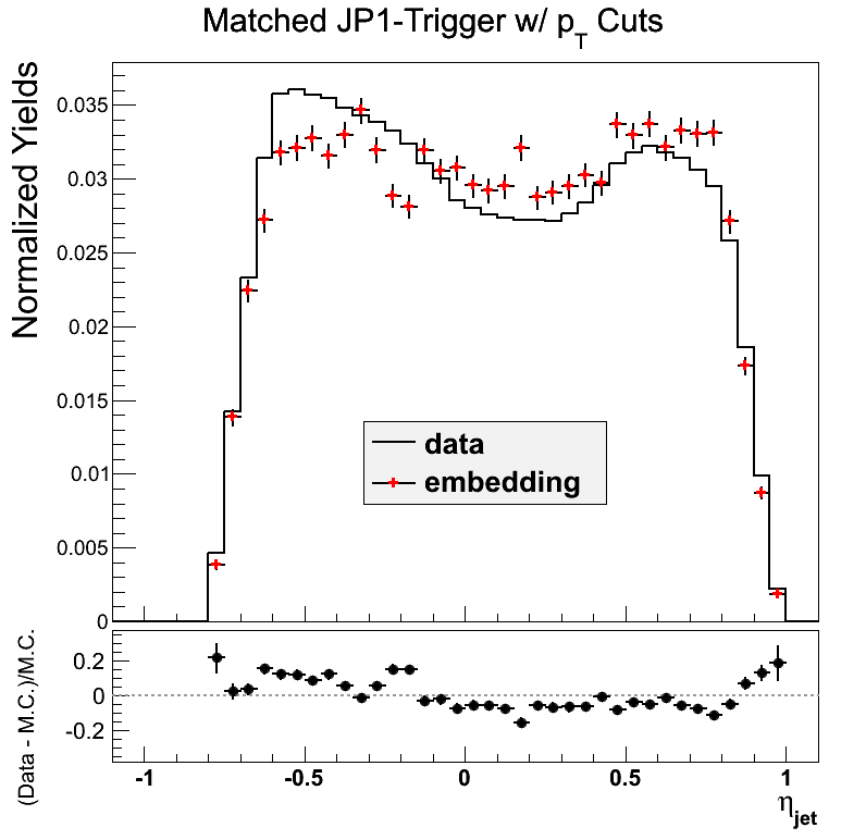
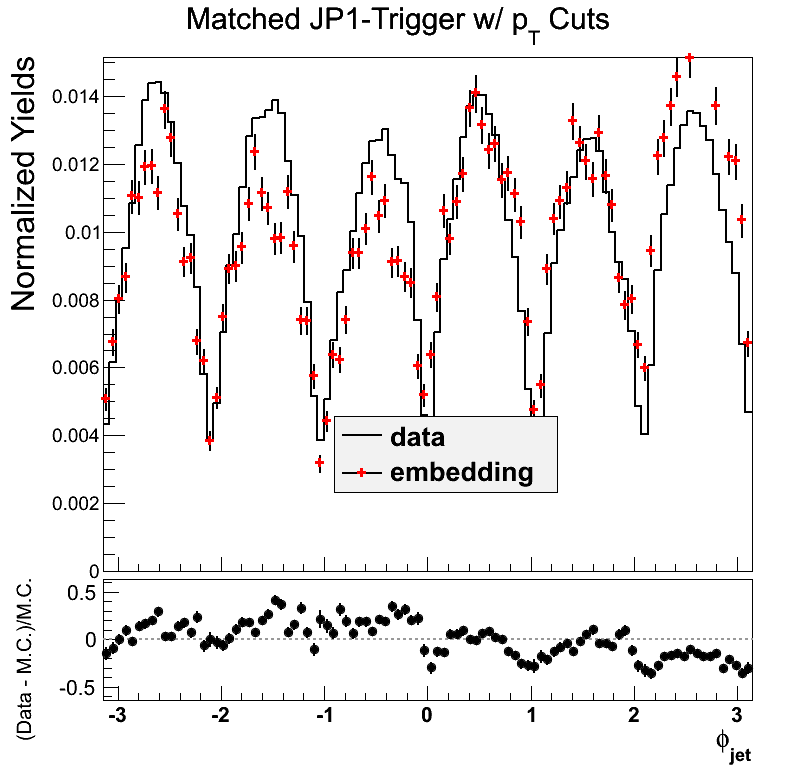
Again, the eta comparison is a bit off near -0.5 in JP1, but not as bad as JP0. The trigger response in phi appears much better, as well, though not perfect by any means.

Figure 10

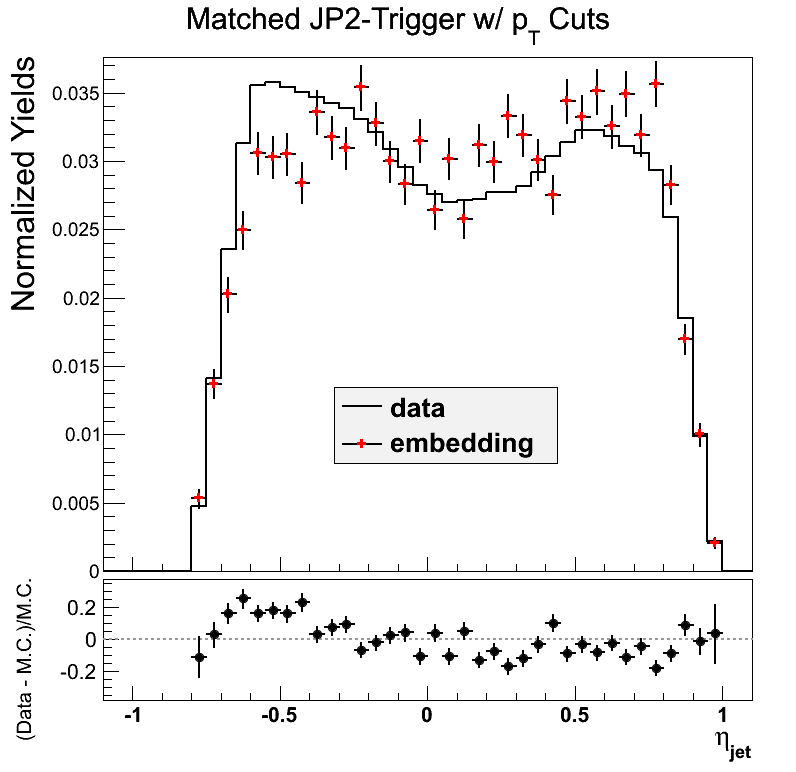
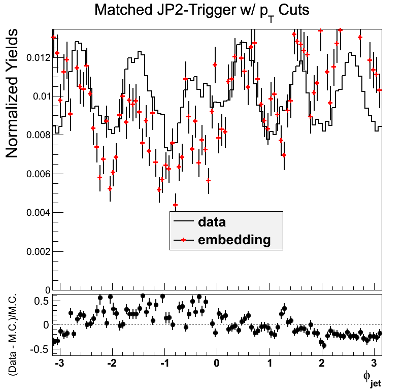
Here, I show JP2 for the new sample (<25 GeV/c in partonic p_T). The eta-phi comparisons in JP2 are similar to that of JP1. The statitistics are lower, so there appear to be more fluctuations.

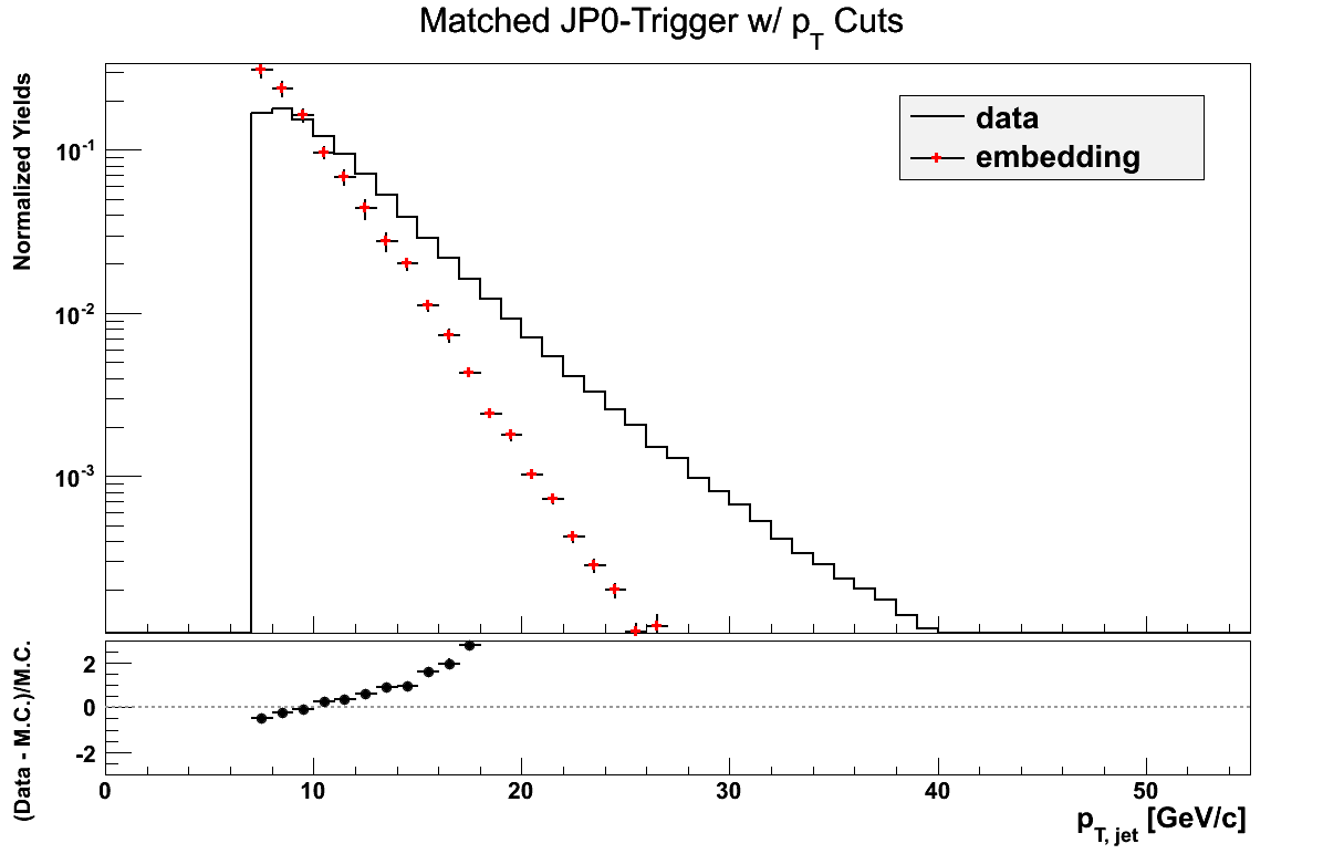
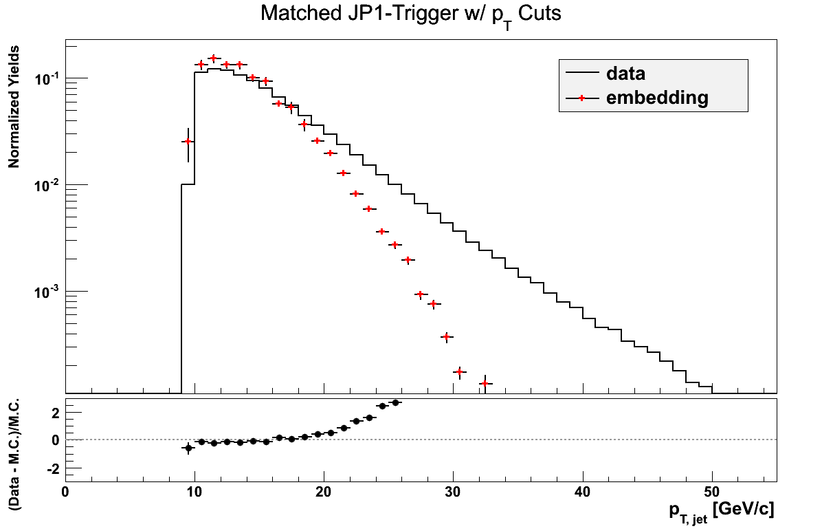
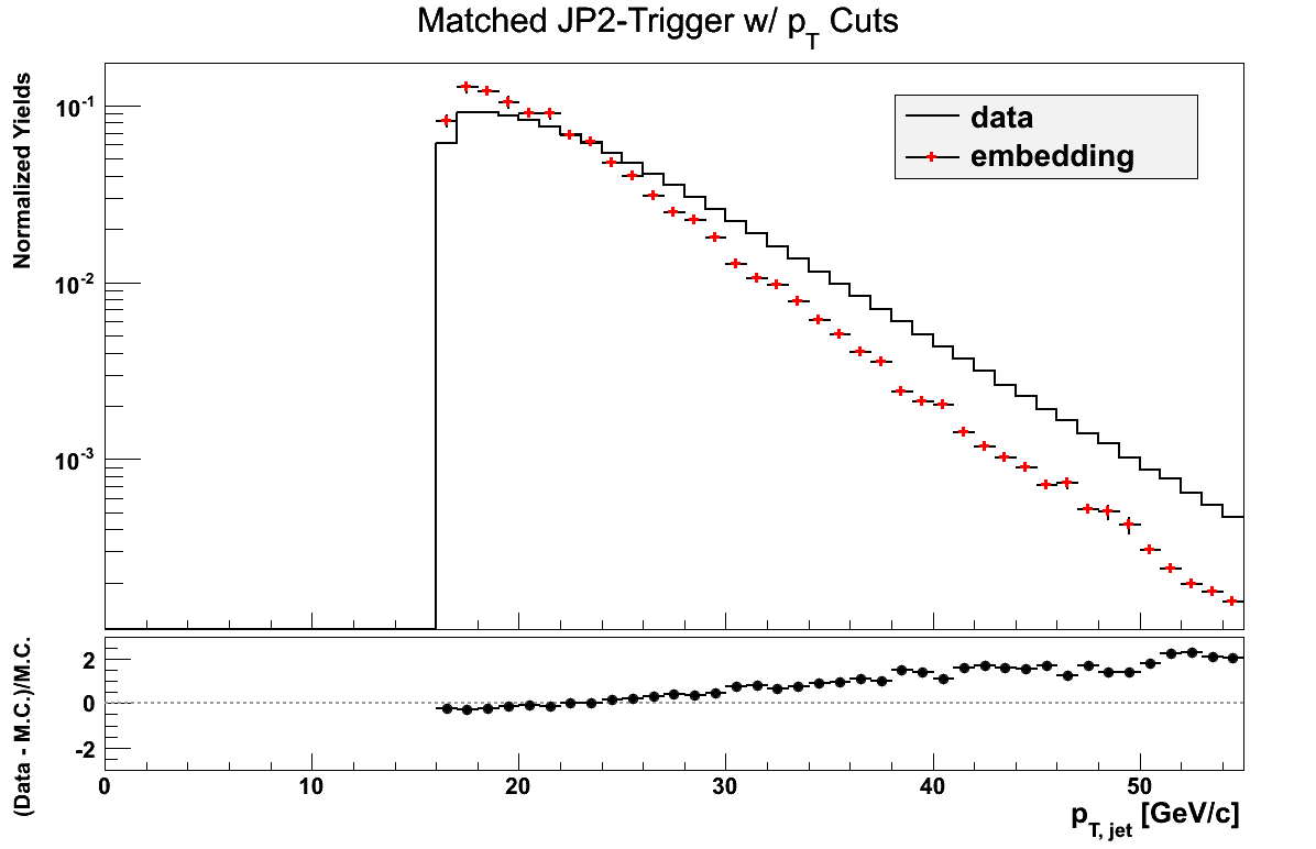
p_T Comparison

Reconstructed jet p_T may not be quite fair at this point, given the differences in how I define my triggers. It may be more relevant to look at a sum over jet triggers. For the moment, I simply look at the comparison of the different triggers, broken down by the aforementioned definitions, bearing in mind the somewhat apples-to-oranges nature. Embedding jets are matched to particle jets.

Figure 10

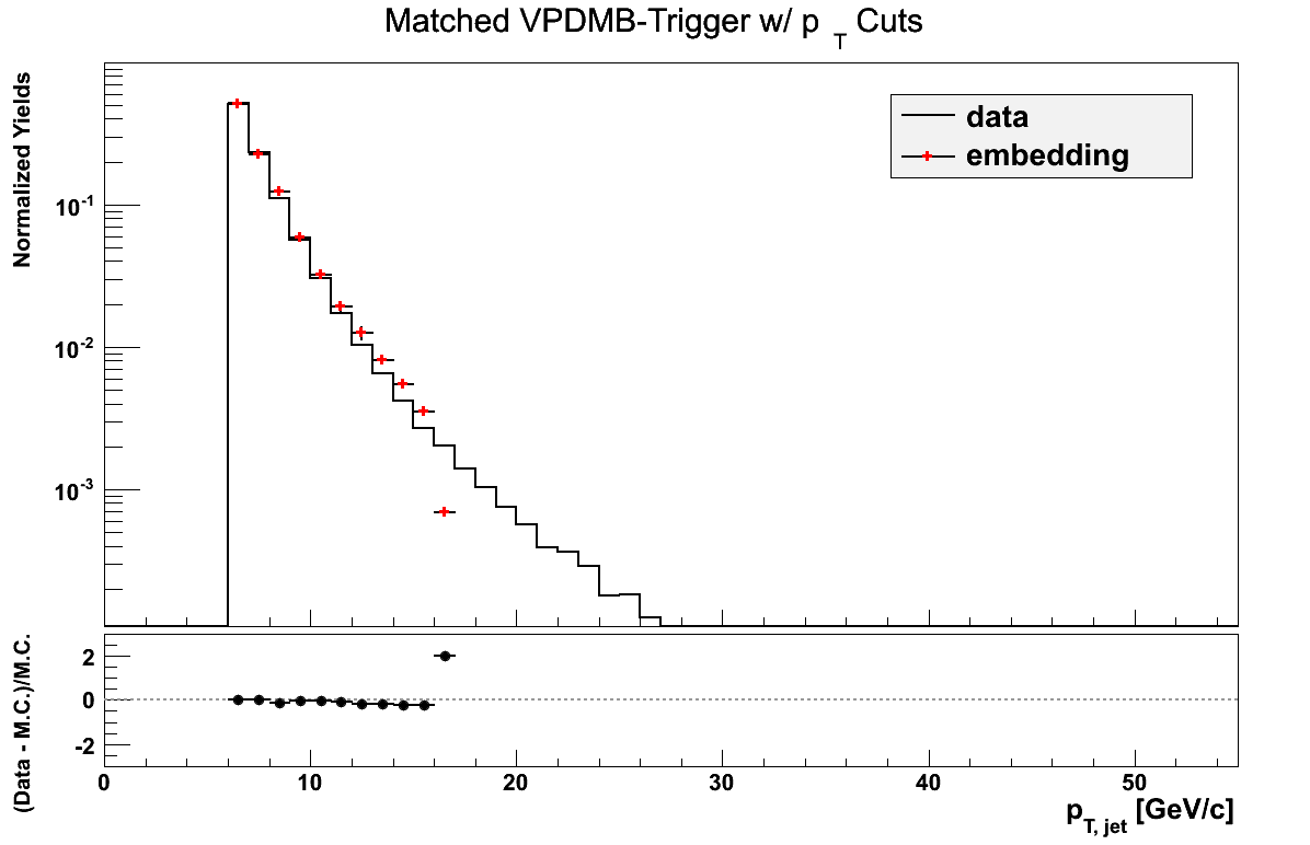
Figure 11