- drach09's home page
- Posts
- 2022
- 2020
- June (1)
- 2019
- 2018
- 2017
- 2016
- 2015
- 2014
- December (13)
- November (2)
- October (5)
- September (2)
- August (8)
- July (9)
- June (7)
- May (5)
- April (4)
- March (4)
- February (1)
- January (2)
- 2013
- December (2)
- November (8)
- October (5)
- September (12)
- August (5)
- July (2)
- June (3)
- May (4)
- April (8)
- March (10)
- February (9)
- January (11)
- 2012
- 2011
- October (1)
- My blog
- Post new blog entry
- All blogs
2006 EEMC Neutral Pions: Updated Systematics
Updated Systematics and Methodology
After an overhaul of my asymmetry calculation and systematics I post new money plots. I summarize the changes as the following:
- Extract raw asymmetry, ε, from p0+p1×sin(φS) fit
- Apply background correction (removal of background asymmetry and scaling for signal fraction) to extracted, raw p1 from fit
- The statistical uncertainty due to the polarization uncertainty (negligible) has been removed from the calculation to be cited as a ~5% scale systematic (correlated across all bins)
- The statistical uncertainty due to the signal fraction uncertainties (propagated fit parameters and residuals) have been moved from statistical to systematic
- The statistical uncertainty due to the background asymmetry uncertainty (changed to 1.2% for both blue and yellow) has been moved from statistical to systematic
- The systematic uncertainty due to the alternative background asymmetry has been removed
- The systematic uncertainty due to the alternative mass window has been removed
Residuals
I have unsuccessfully attempted to recalculate by hand the content stored in hCountsSysUncertResFit. I summarize my attempt for xF bin-1 as the following
- Fit a constant to res_1 from 0.1 to 0.2 GeV/c2 to obtain 45.97±35.99
- Scale by the number of bins to obtain 919.4±719.8
- Scale by the bin width (0.05) to obtain 45.97±35.99
Figure 1
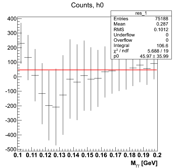
This does not correspond to the 9.84 found via hCountsSysUncertResFit->GetBinContent(1). It is not clear to me that scaling by the bin width is the right thing to do, but perhaps we can clear that up in the meeting. If I simply take the bin sums I obtain 106.6, which if I scale by the bin width becomes 5.33. For the following figures I simply take the sum across the bins (106.6 in this particular xF bin).
Calculation
AN = ( (1/P)×ε-(1-fsig)×AN, bg )/fsig
(δAN)stat = ( (1/P)×δε )/fsig
(δAN)bg = ( (1-fsig)/fsig )×δAN, bg
(δAN)sig. frac. prop = (AN-AN, bg)×(δfsig, prop/fsig)
(δAN)sig. frac. res = (AN-AN, bg)×(δfsig, res/fsig)
(δAN)syst = √( (δAN)bg2 + (δAN)sig. frac. prop2 + (δAN)sig. frac. res2 )
Money Plots
Figure 2
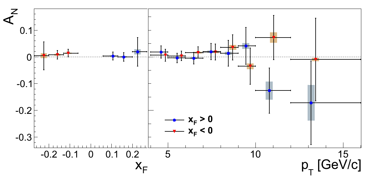
Figure 3
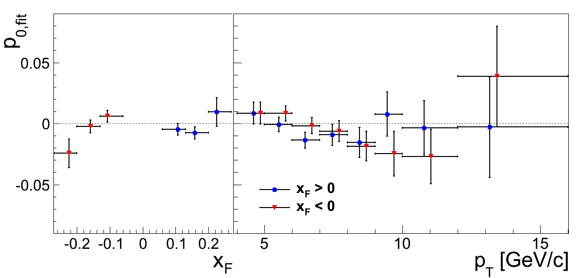
Table 1: xF > 0
| ε | ε stat error | AN | AN stat err | AN stat err CR | AN stat err Pol | AN total Syst | AN syst err fit-prop | AN syst err fit res | AN syst B.g. AN | AN Mass Win. Cross-check | |
|---|---|---|---|---|---|---|---|---|---|---|---|
| xF Bin 1 | 0.001786 | 0.006825 | 0.003010 | 0.014597 | 0.014597 | 0.000141 | 0.001963 | -0.000077 | -0.000006 | 0.001961 | -0.000188 |
| xF Bin 2 | 0.000509 | 0.006999 | -0.000117 | 0.016238 | 0.016238 | -0.000005 | 0.003163 | -0.000327 | -0.000104 | 0.003145 | -0.006592 |
| xF Bin 3 | 0.006957 | 0.016502 | 0.018700 | 0.053226 | 0.053226 | 0.000879 | 0.009739 | 0.003574 | 0.000323 | 0.009054 | -0.028404 |
| pT Bin 2 | 0.009429 | 0.012402 | 0.017415 | 0.022950 | 0.022950 | 0.000819 | 0.000618 | 0.000535 | -0.000300 | 0.000080 | 0.009248 |
| pT Bin 3 | -0.001749 | 0.008387 | -0.004502 | 0.017844 | 0.017844 | -0.000212 | 0.001996 | -0.000627 | -0.000152 | 0.001889 | -0.008215 |
| pT Bin 4 | -0.001423 | 0.009225 | -0.004739 | 0.021716 | 0.021716 | -0.000223 | 0.003465 | -0.000791 | -0.000228 | 0.003366 | -0.001287 |
| pT Bin 5 | 0.008464 | 0.012130 | 0.019343 | 0.030253 | 0.030253 | 0.000909 | 0.004539 | 0.001504 | 0.000134 | 0.004281 | -0.010235 |
| pT Bin 6 | 0.005614 | 0.017319 | 0.013122 | 0.048455 | 0.048455 | 0.000617 | 0.006444 | 0.001515 | 0.000050 | 0.006263 | -0.003482 |
| pT Bin 7 | 0.015997 | 0.025662 | 0.040618 | 0.068806 | 0.068806 | 0.001909 | 0.010842 | 0.009334 | -0.000389 | 0.005502 | -0.011237 |
| pT Bin 8 | -0.045464 | 0.030793 | -0.126508 | 0.084057 | 0.084057 | -0.005946 | 0.034284 | -0.033782 | -0.000573 | 0.005819 | -0.041647 |
| pT Bin 9 | -0.063955 | 0.058972 | -0.172061 | 0.156623 | 0.156623 | -0.008087 | 0.066870 | -0.066511 | 0.004401 | 0.005337 | -0.062893 |
Table 2: xF < 0
| ε | ε stat error | AN | AN stat err | AN stat err CR | AN stat err Pol | AN total Syst | AN syst err fit-prop | AN syst err fit res | AN syst B.g. AN | AN Mass Win. Cross-check | |
|---|---|---|---|---|---|---|---|---|---|---|---|
| xF Bin 1 | 0.006411 | 0.006824 | 0.013512 | 0.014385 | 0.014385 | 0.000649 | 0.002033 | 0.000536 | 0.000039 | 0.001961 | 0.000621 |
| xF Bin 2 | 0.003399 | 0.006999 | 0.007771 | 0.016002 | 0.016002 | 0.000373 | 0.003188 | 0.000500 | 0.000160 | 0.003145 | 0.001433 |
| xF Bin 3 | 0.001181 | 0.016486 | 0.003755 | 0.052405 | 0.052405 | 0.000180 | 0.009107 | 0.000976 | 0.000088 | 0.009054 | 0.058065 |
| pT Bin 2 | 0.003333 | 0.012402 | 0.006079 | 0.022618 | 0.022618 | 0.000292 | 0.000309 | 0.000261 | -0.000146 | 0.000080 | 0.008343 |
| pT Bin 3 | 0.001582 | 0.008385 | 0.003316 | 0.017583 | 0.017583 | 0.000159 | 0.001902 | 0.000220 | 0.000053 | 0.001889 | -0.009815 |
| pT Bin 4 | 0.006811 | 0.009224 | 0.015801 | 0.021399 | 0.021399 | 0.000758 | 0.003623 | 0.001289 | 0.000372 | 0.003366 | 0.017972 |
| pT Bin 5 | 0.007356 | 0.012136 | 0.018081 | 0.029831 | 0.029831 | 0.000868 | 0.004682 | 0.001890 | 0.000169 | 0.004281 | 0.000734 |
| pT Bin 6 | 0.012713 | 0.017292 | 0.035055 | 0.047679 | 0.047679 | 0.001683 | 0.009030 | 0.006502 | 0.000216 | 0.006263 | 0.003563 |
| pT Bin 7 | -0.013361 | 0.025672 | -0.035305 | 0.067837 | 0.067837 | -0.001695 | 0.010761 | -0.009240 | 0.000385 | 0.005502 | -0.032221 |
| pT Bin 8 | 0.026638 | 0.030765 | 0.071662 | 0.082766 | 0.082766 | 0.003440 | 0.019315 | 0.018415 | 0.000312 | 0.005819 | 0.077817 |
| pT Bin 9 | -0.003934 | 0.059059 | -0.010297 | 0.154585 | 0.154585 | -0.000494 | 0.006597 | -0.003869 | 0.000256 | 0.005337 | 0.075118 |
Mass Window
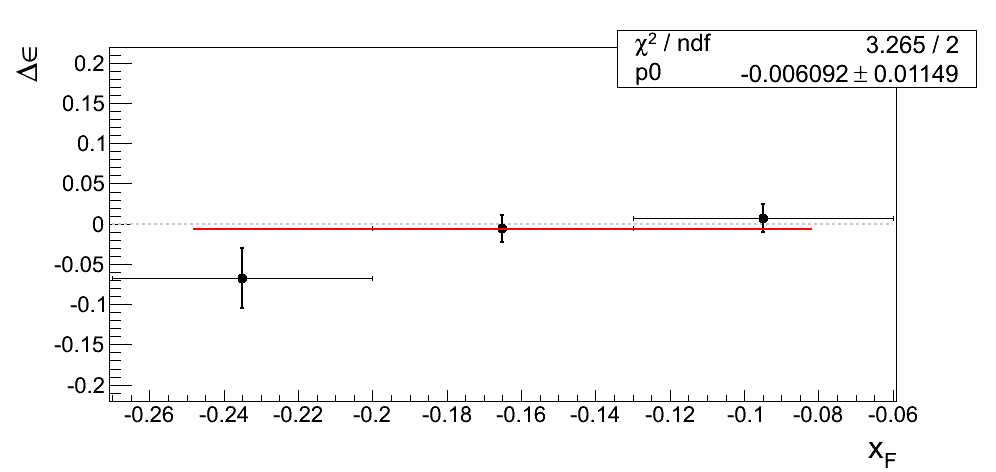
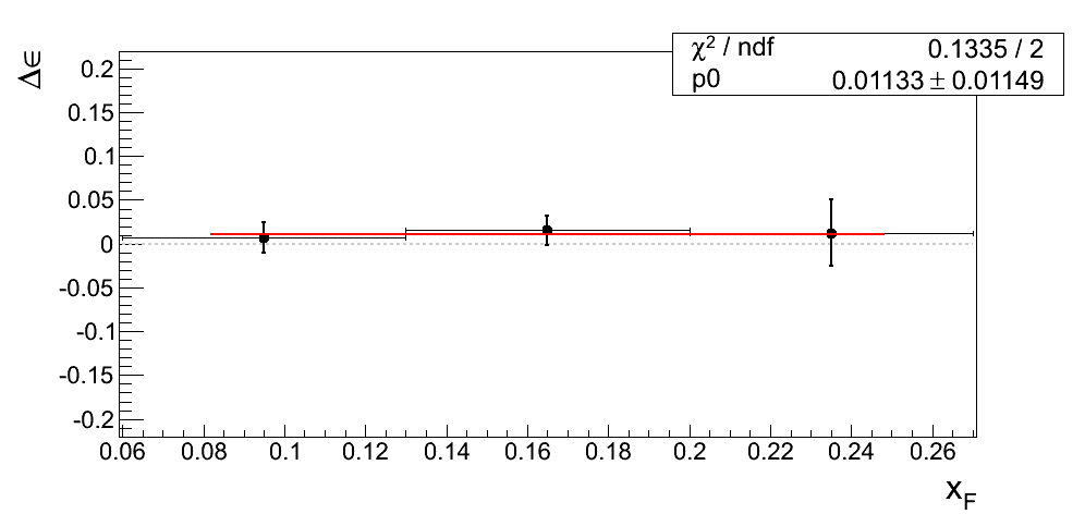
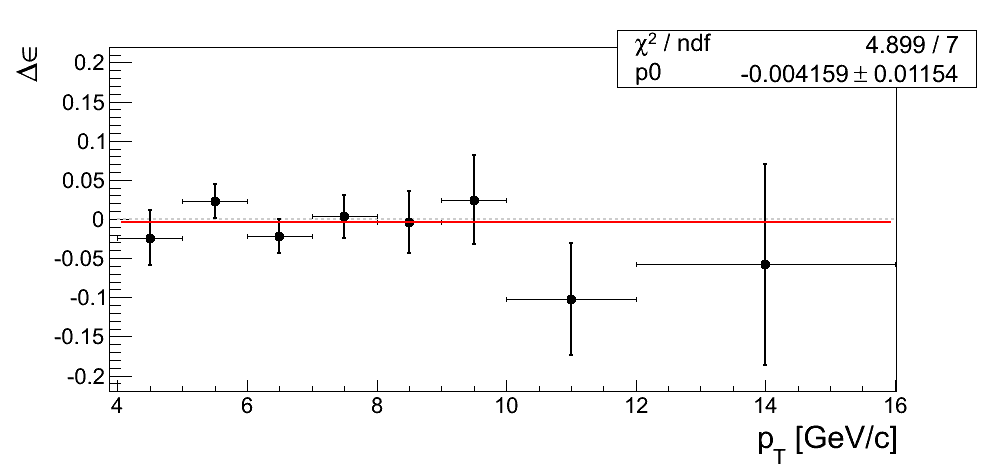
Our decision to drop the mass-window systematic is justified only if we can demonstrate the differences from our nominal window are dominated by statistics. In Fig. 4 I post the difference between ε extraction from the tight mass window and the high-mass band. The difference is fit with a constant.
Figure 4
| xF < 0 | xF > 0 |
|---|---|
 |
 |
 |
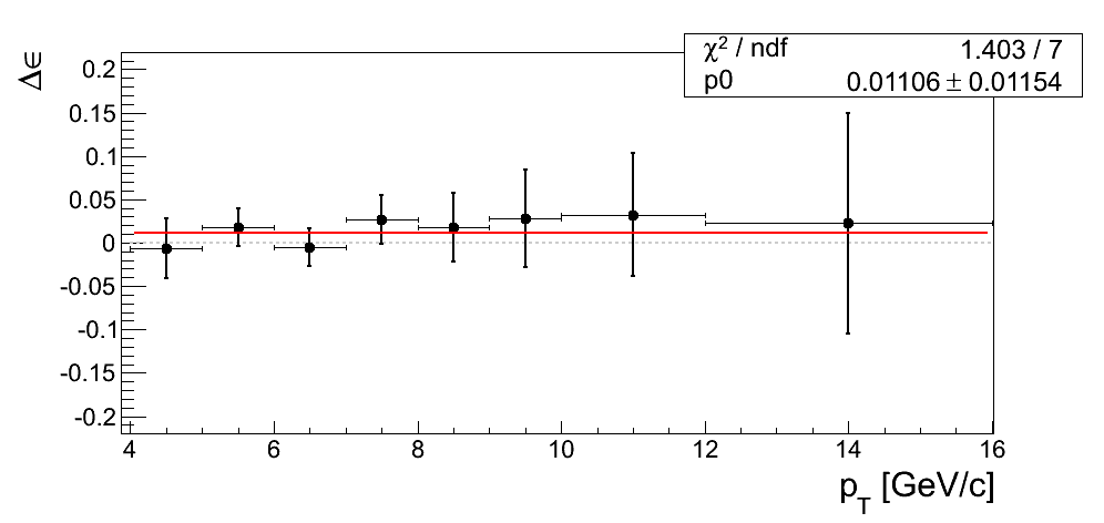 |
In all cases the constant returns a value within 1σ of zero. Additionally, the χ2/ν values are reasonable. One must remember the events are 100% correlated between the xF binning and the pT binning. While perhaps not compelling, Figure 4 is suggestive that our mass-window cross-check is statistics-dominated.
Comparison to Published Data
Elke had specifically asked for me to post the average pT values for the various xF bins in our comparison plot. I have computed these values for our data, grabbed the published values from the paper, and remade the figure with the latest systematics.
Figure 5
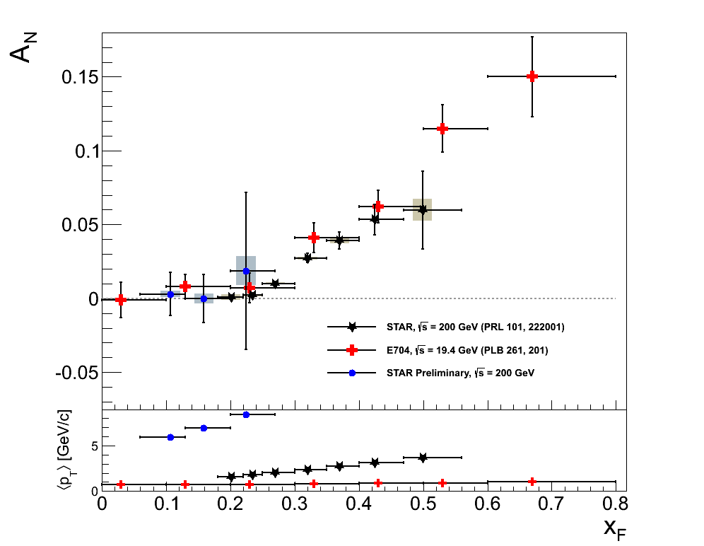
I like this addition in terms of its information. The aesthetics are not quite so pleasing with the E704 data being so low in pT with the given scale. However, the message is clear. The RHIC data push us to significantly higher pT. It is too bad we don't have a factor of 10 more statistics in our third bin!
- drach09's blog
- Login or register to post comments
