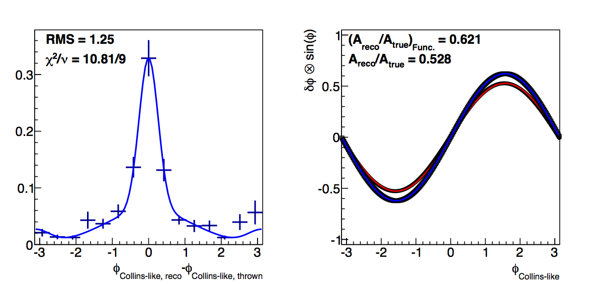
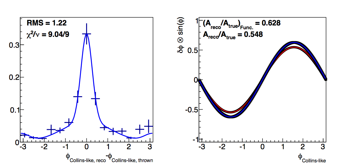
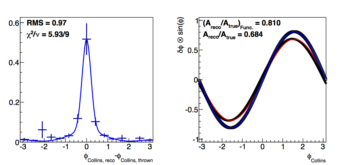
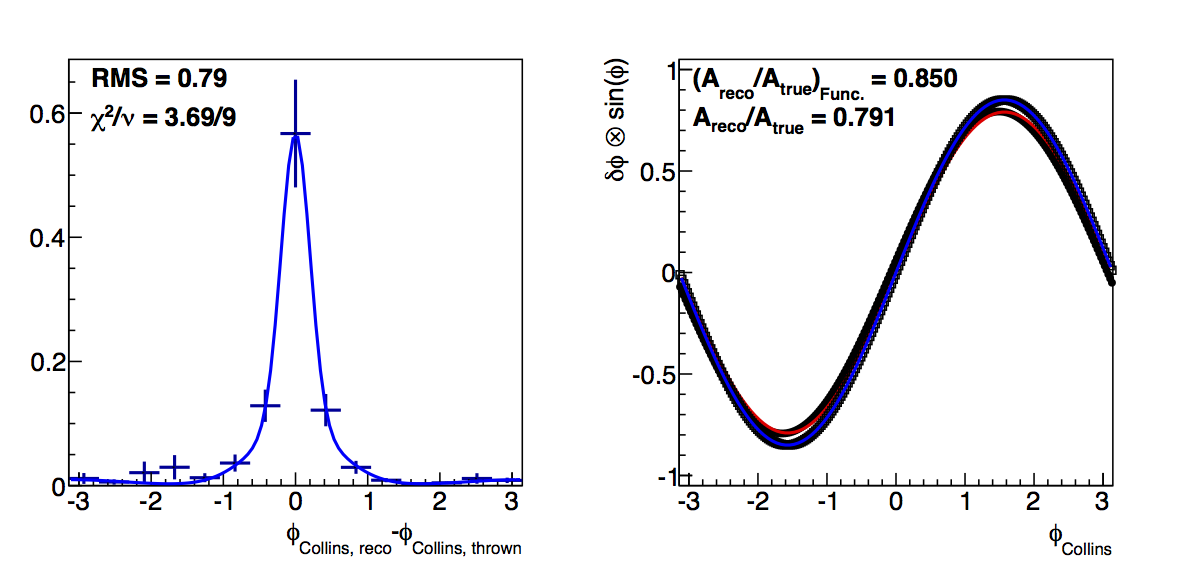
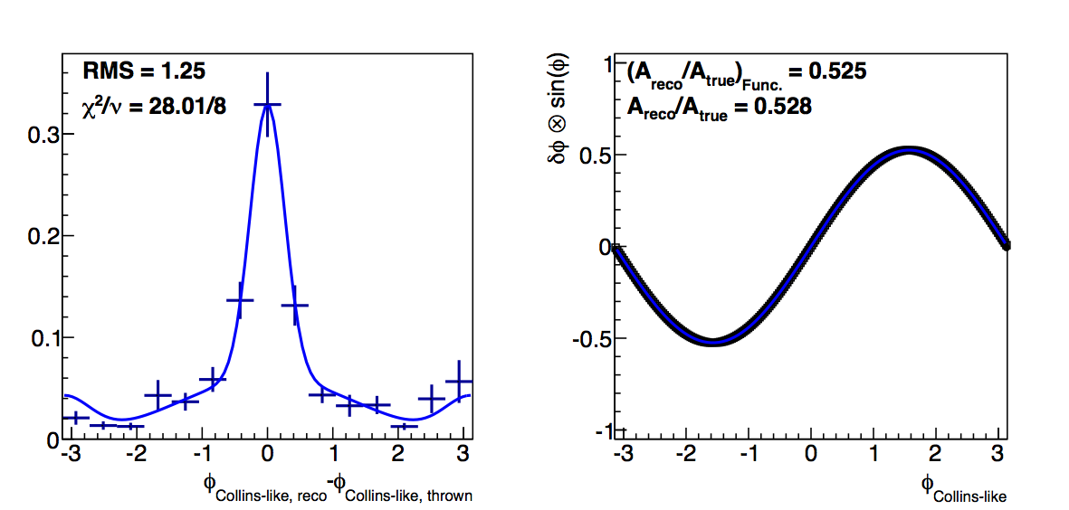
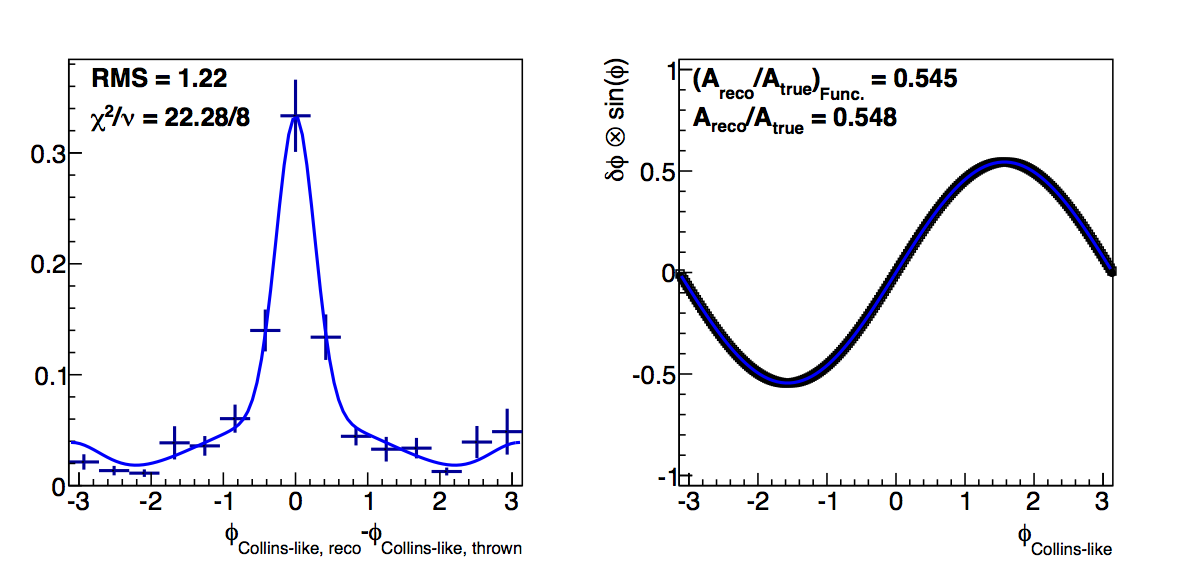
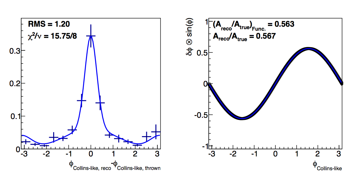
As a follow-up from the jet call, I have revisited the resolution study. Now, I compare the results of convoluting the raw φ_reco-φ_true distributions with sinusoids to convoluting functional fits to the φ_reco-φ_true distributions with sinusoids. The hope is that I can gain an understanding of how the statistical fluctations affect the resolution estimates. It will matter, then, what kind of fit quality I can get to the δφ distributions. Thus, for the fits, I rebin the δφ histograms by a factor of 16 (240 bins to 15 bins). For the raw convolutions, however, I use the original 240 bin versions.

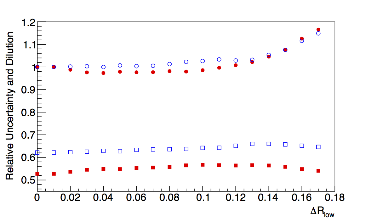
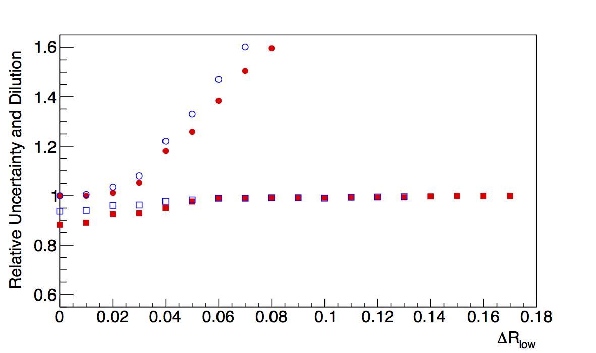
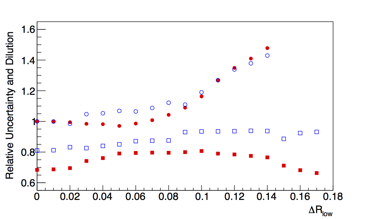
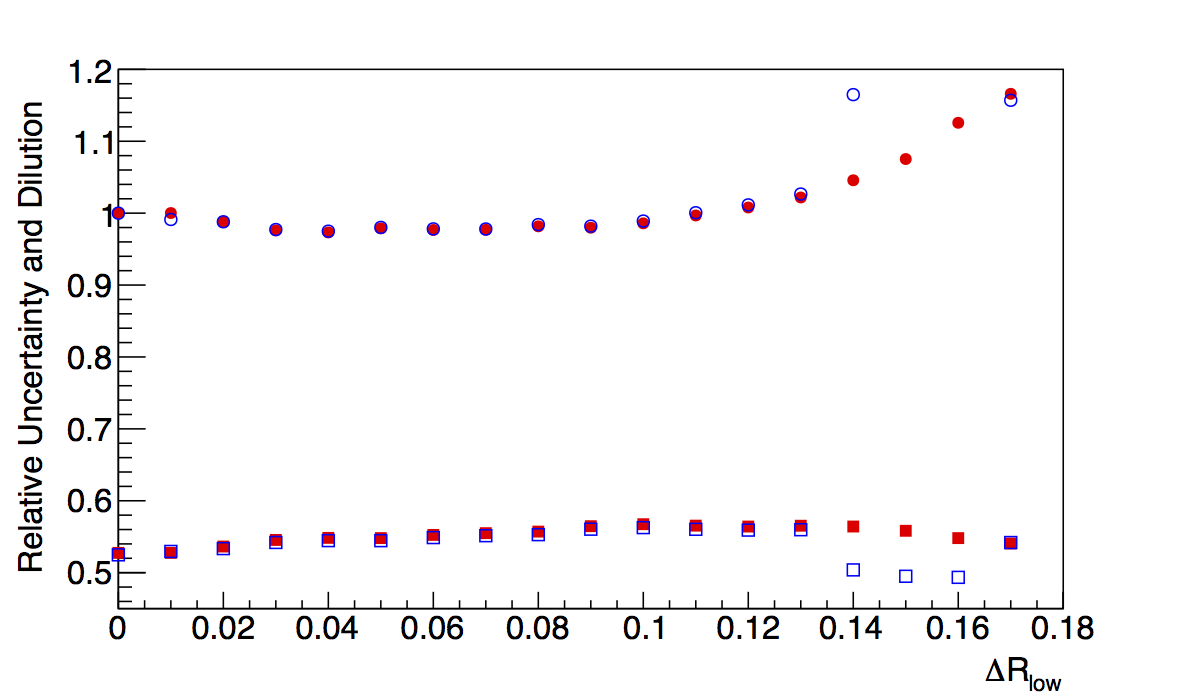
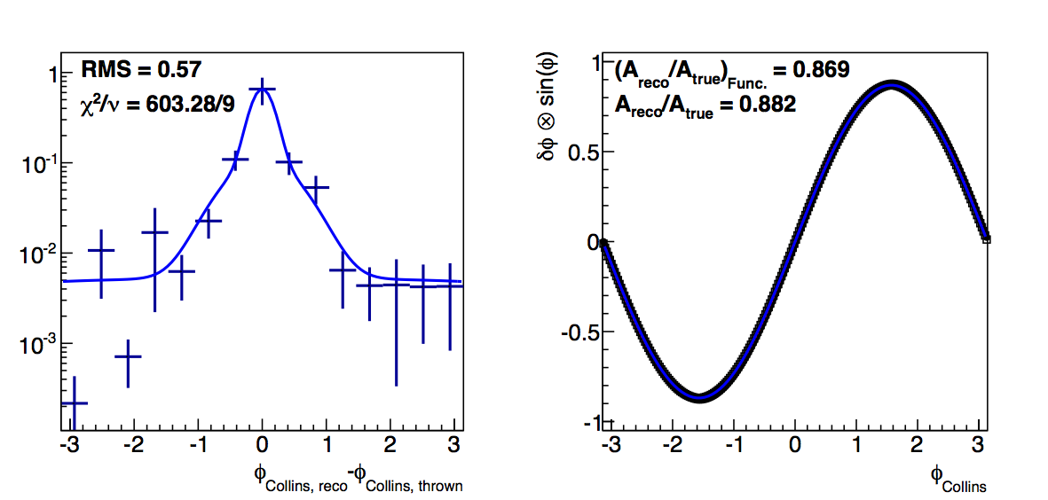
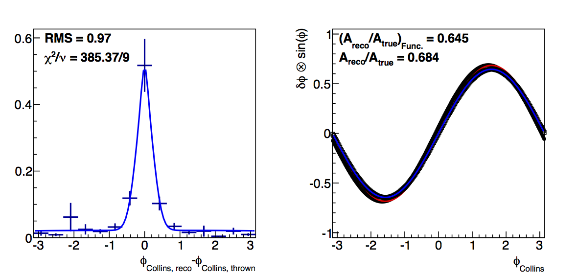
Figure 1: Low-p_T, low-z Collins-like

ΔR > 0	ΔR > 0.05	ΔR > 0.1

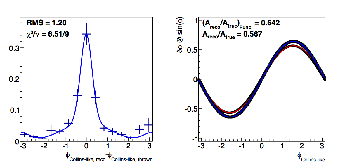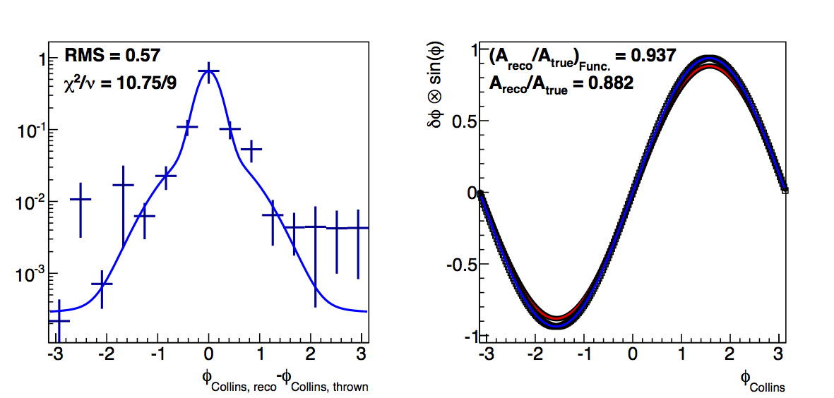
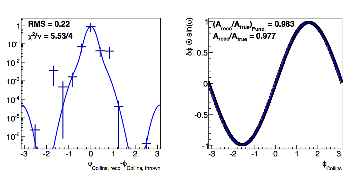
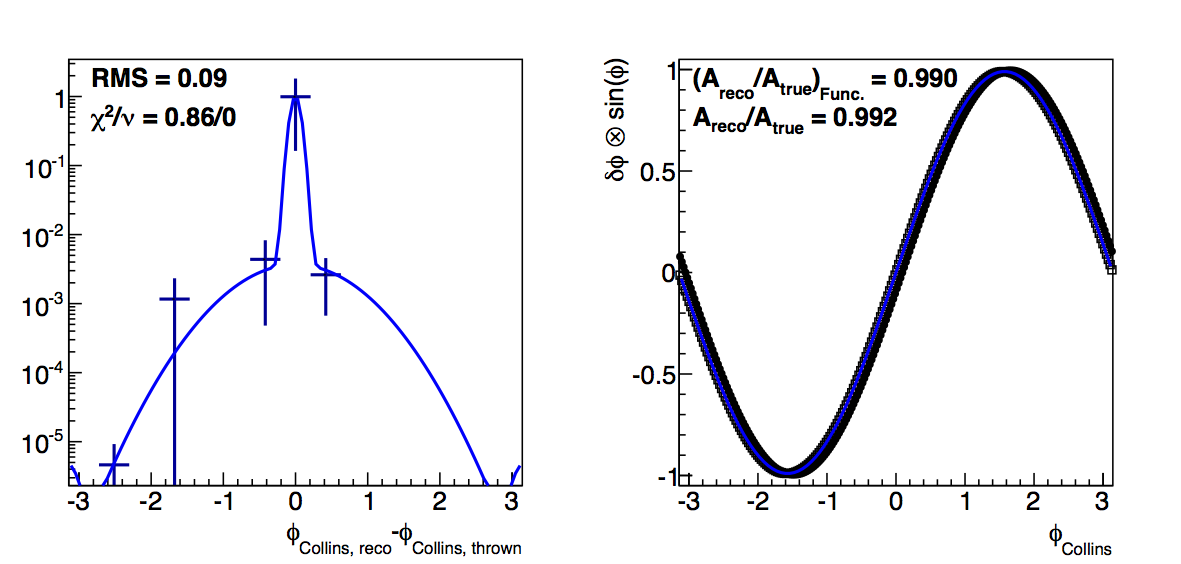
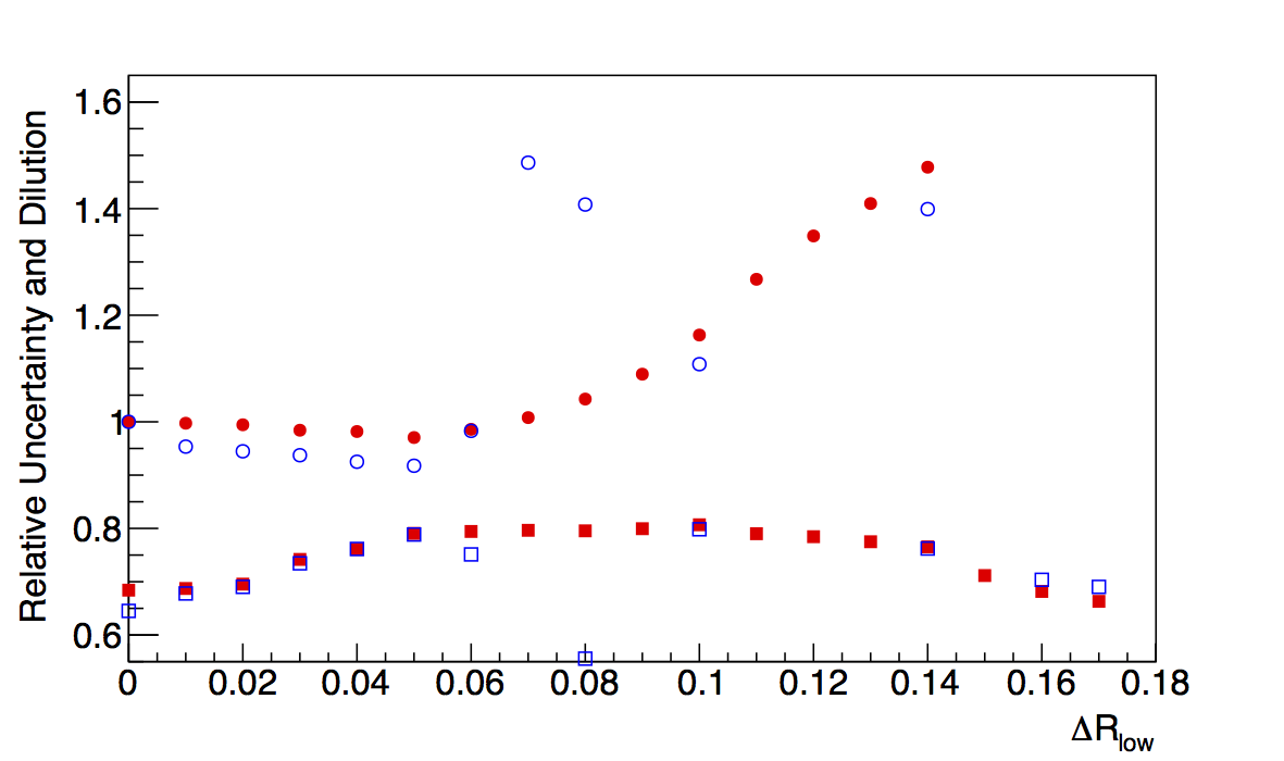
In Fig. 1 I show the results for Collins-like resolutions with VPDMB, 6 < p_T < 7.1 GeV/c, and 0.1 < z < 0.3. In red I plot the "raw" method and in blue the "fit" method. Squares are the dilution factors and circles are the relative uncertainties. I manage to get fairly decent fits using a three-Gaussian function (two centered at zero and one at π). Across the board, the functional forms result in smaller dilutions. I believe this to be the result of smoothing out the statistical fluctuations, e.g. around δφ ~ -2 and 3. 

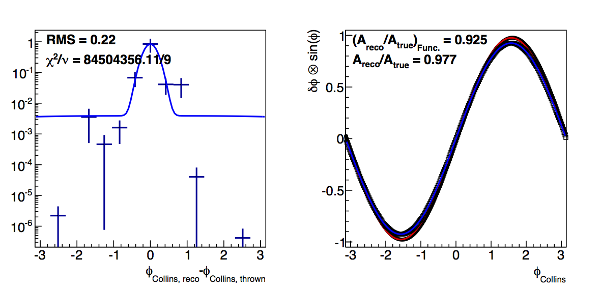
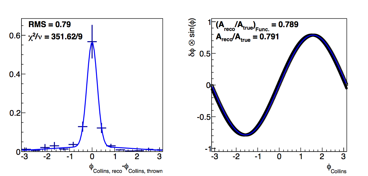
Figure 2: High-p_T, high-z Collins

ΔR > 0	ΔR > 0.05	ΔR > 0.1

In Fig. 2, I show the results for Collins resolutions from JP2 with 22.7 < pT < 26.8 GeV/c and z > 0.3. Here, the differences are much smaller between the raw and fit methods. Note how quickly the statistics really die off as one increases the radius cut. This further argues that we should loosen the radius cut, so that we can ensure sufficient embedding statistics for a robust correction.

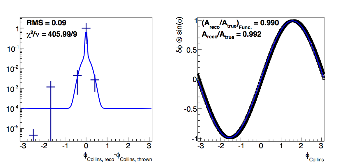
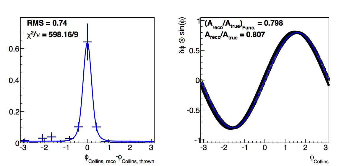
Figure 3: Low-p_T, high-z Collins

ΔR > 0	ΔR > 0.05	ΔR > 0.1

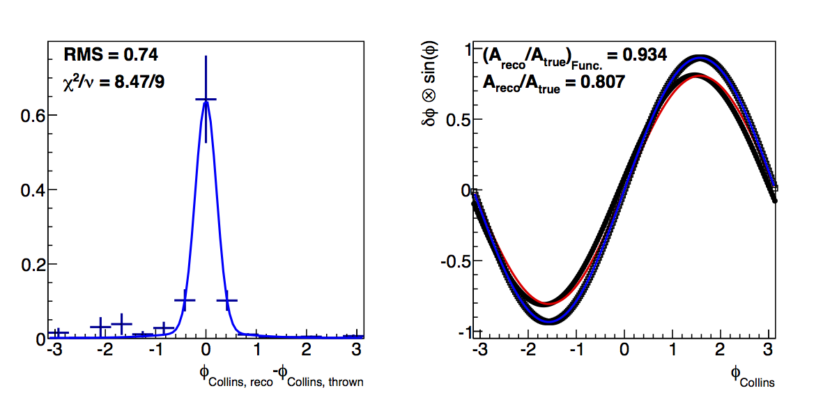In Fig. 3 I show the results for Collins resolutions from VPDMB with 6 < pT < 7.1 GeV/c and z > 0.3. Here, again, the fit method results in smaller dilutions than the raw convolution method. Also, the resolution seems to stablize as the cut increases in contrast to the fall-off from teh raw method. Again, I attribute the smaller dilutions to the fit method smoothing out statistical fluctuations.

Where to?

The conclusions do not seem to change from the previous study. I still argue that relaxing the radius cut to 0.05 is reasonable. Going forward, I am a bit nervous about the effect of the statistical fluctuations. One reasonable path forward may be to use the fit method to derive the correction to ensure that the fluctuations do not hurt us. Then, we can take the difference from the raw convolution as a systematic, i.e. A×(σ_D/D), where σ_D is the difference between the "fit" dilution and the "raw" dilution.

Log Likelihood

Carl has suggested that the fits may systematically undershoot the high-δφ points, causing the lower dilution in the fit method. Adding a constant term to the fits does not seem to improve them. As another check, I have switched to the log-likelihood fitting method to see if the fits change.

Figure 4: Low-p_T, Low-z Collins-like

ΔR > 0	ΔR > 0.05	ΔR > 0.1

Changing to the log-likelihood method certainly seems to change things. Now, the "fit" method returns almost identically the "raw" dilutions. The χ²s for the fits are obviously not as good, but the fit does seem more effectively to account for the high-δφ points (though undershooting the low-δφ points).

Figure 5: High-p_T, high-z Collins

ΔR > 0	ΔR > 0.05	ΔR > 0.1

Again, changing to log-likelihood, now, better accounts for the high-δφ points. In the high-p_T, high-z case, the methods returned fairly close values, anyway. The log-likelihood case is different only in that the "fit" method actually returns lower resolutions.

Figure 6: Low-p_T, high-z Collins

ΔR > 0	ΔR > 0.05	ΔR > 0.1

In the low-p_T, high-z case, the log-likelihood fits, again, improve the agreement between the fit and raw methods. This is undoubtedly from the better fitting to the high-δφ points. Certainly, the χ² quality is not as high, but it may argue that in this case, the log-likelihood method is more appropriate.