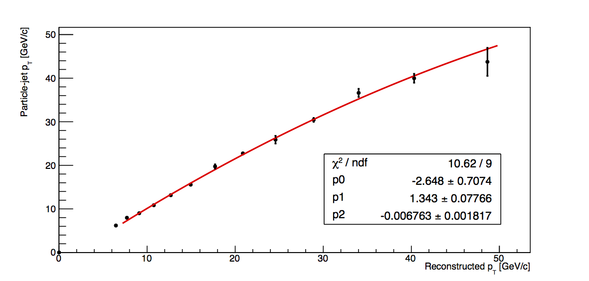
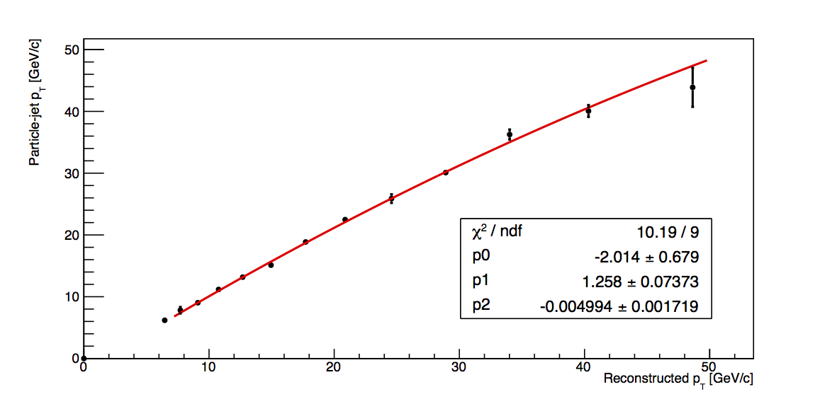
Given the limitations of my embedding sample, it is important to try to use the available statistics most efficiently. One way to do this is to utilize fits to the data trends. Rather than simply taking the calculated means and uncertainties at face value, I can look at the relationship, e.g., of corrected p_T to reconstructed p_T. Then, I can use the fit curves to calculated an alternative kinematic shift which maximizes the availble precision.

After tuning the hadron radius cut, I have sufficient embedding statistics that my z and jT shifts are quite fine without the fitting. The jet p_T in bins of pion z, however, can still use a bit of smoothing. Below, I outline the specifics of my procedure.

• Plot particle-jet p_T vs. detector-jet p_T and fit with a quadratic across the range of 7 < p_T,reco < 50 GeV/c (since the 6-7.1 GeV/c bin is fully VPDMB, I do not expect it to follow the same trend as those points which contain largely JP-triggers)
• Calculate corrected p_T as p₀+p_T,det×p₁+p_T,det²×p₂
• Calculate the square of the fit uncertainty, σ_fit², from the covariance matrix, covMat, as σ_fit² = covMat(0,0)+p_T,det²×covMat(1,1)+p_T,det⁴×covMat(2,2)+2×[p_T,det×covMat(0,1) + p_T,det²×covMat(0,2) + p_T,det³×covMat(1,2)]

Figure 1: Particle-jet p_T vs. Detector-jet p_T

ADC, Track Eff.	Mid-z	High-z
+3, 100%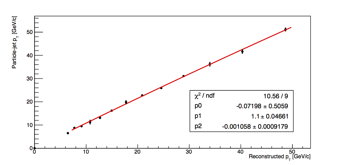
+0, 100%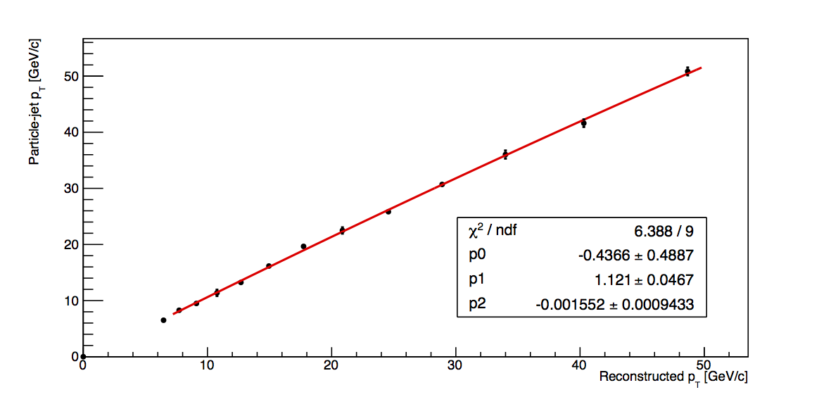
+3, 93%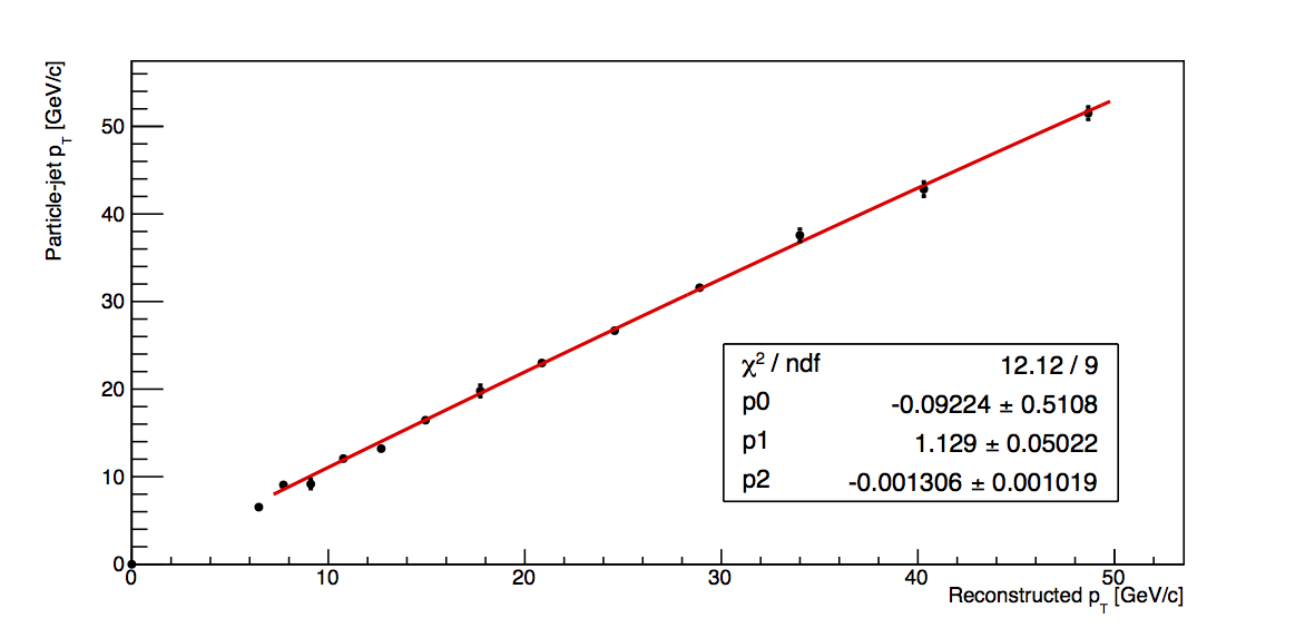

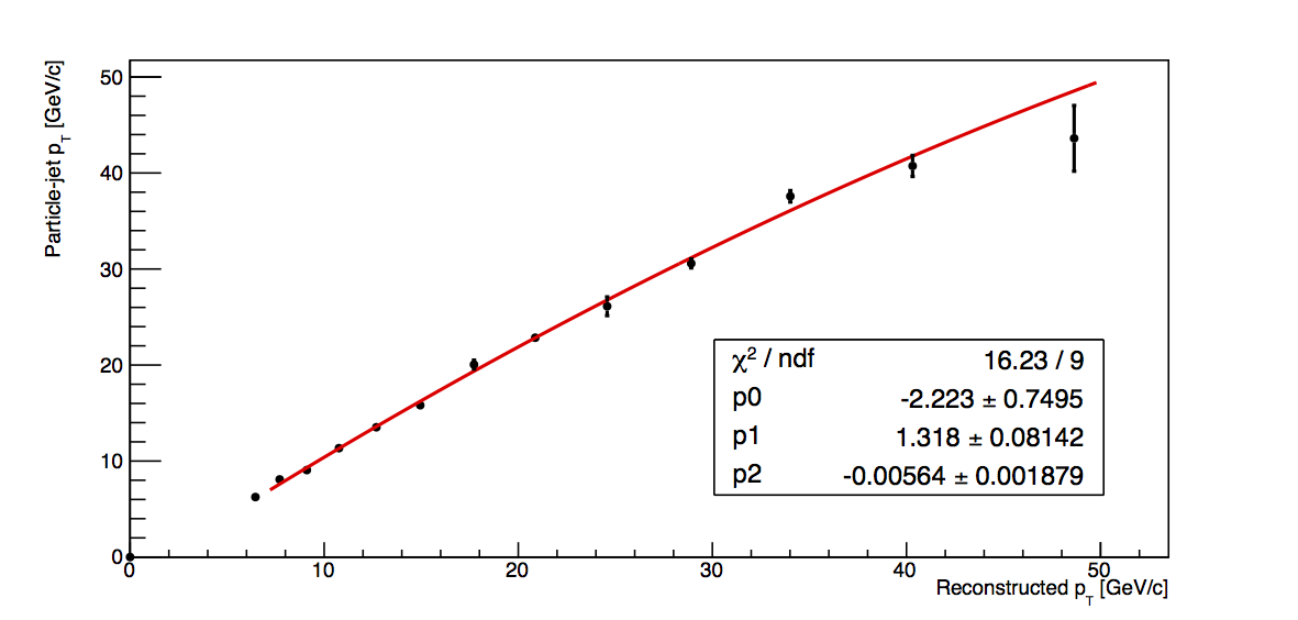The fit results are shown in Fig. 1. In all cases, the quadratic fits the data quite nicely. This suggests that the fit function is reasonable and that calculating the corrections via the fit method may be a valid way to proceed.

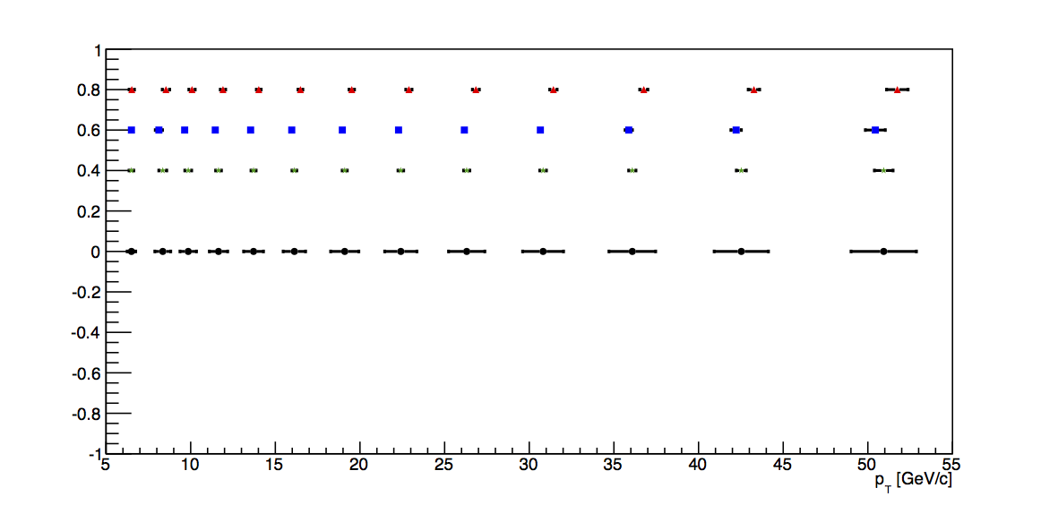
Figure 2

Mid-z	High-z

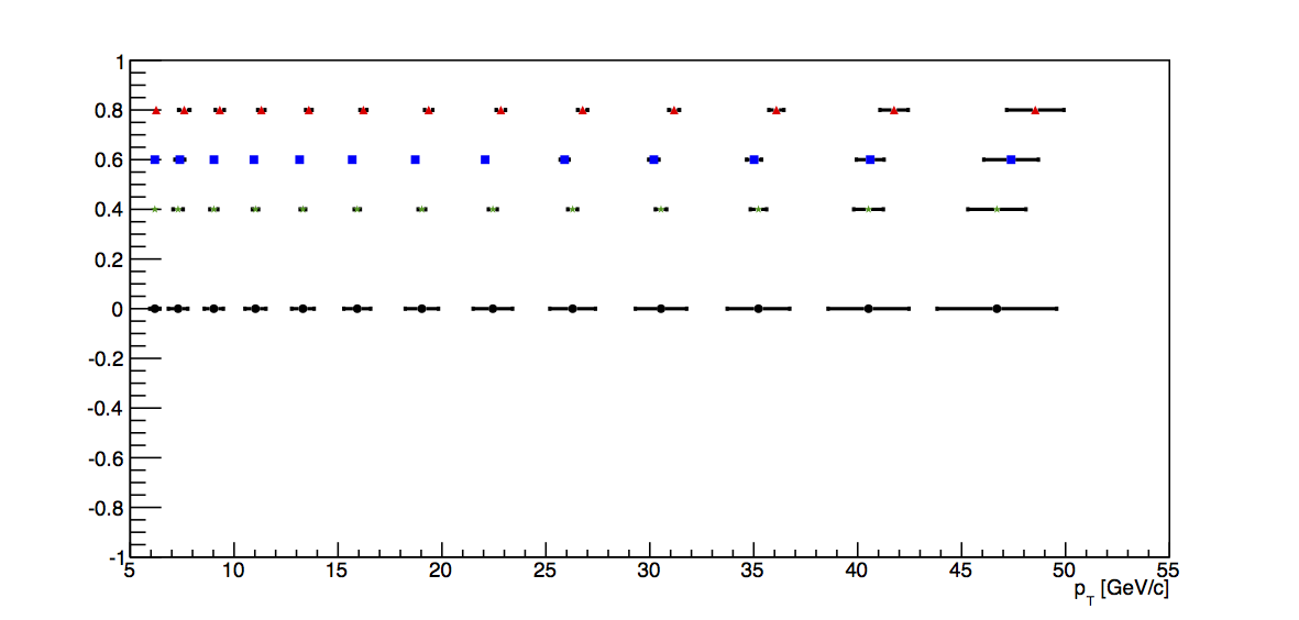In Fig. 2, I show the final, corrected p_Ts with their total systematic uncertainties. In green, I plot the ADC+3, 100% value with their statistical uncertainties, in blue the ADC+0, 100% values, and in red the ADC+3, 93% values.