The comparison between jets created from the Run 9 pp500 data and from the detector level embedded simulation has displayed excellent agreement. The next step moving forward is to determine the corrections need to move from the detector level to the particle level.  It is important to note that we are using the standard cuts implemented for dijet selection and only analyze jets which have a reconstructed geant jet matched to a particle jet. The latter condition is obtained by requiring the difference in the jet axises be less than 0.2 (dR < 0.2*) . We examine the distributions of the invariant mass (Imass) of the dijets for the detector level vs the particle level (Fig 3.).

                              Figure 1: The spectrum of the difference of the between the particle and detector jet 3 radii (JP2)

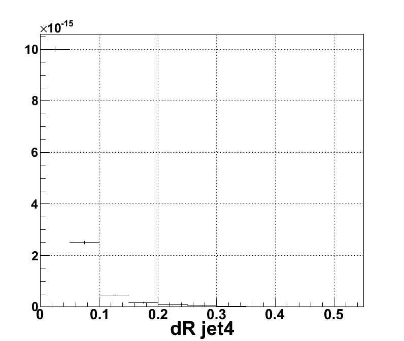
                                  Figure 2: The spectrum of the difference of the between the particle and detector jet 4 radii (JP2)

* This cut is open to change to an optimal values

                                             Figure 3: The detetector level vs the particle level invariant mass spectrum (JP2)

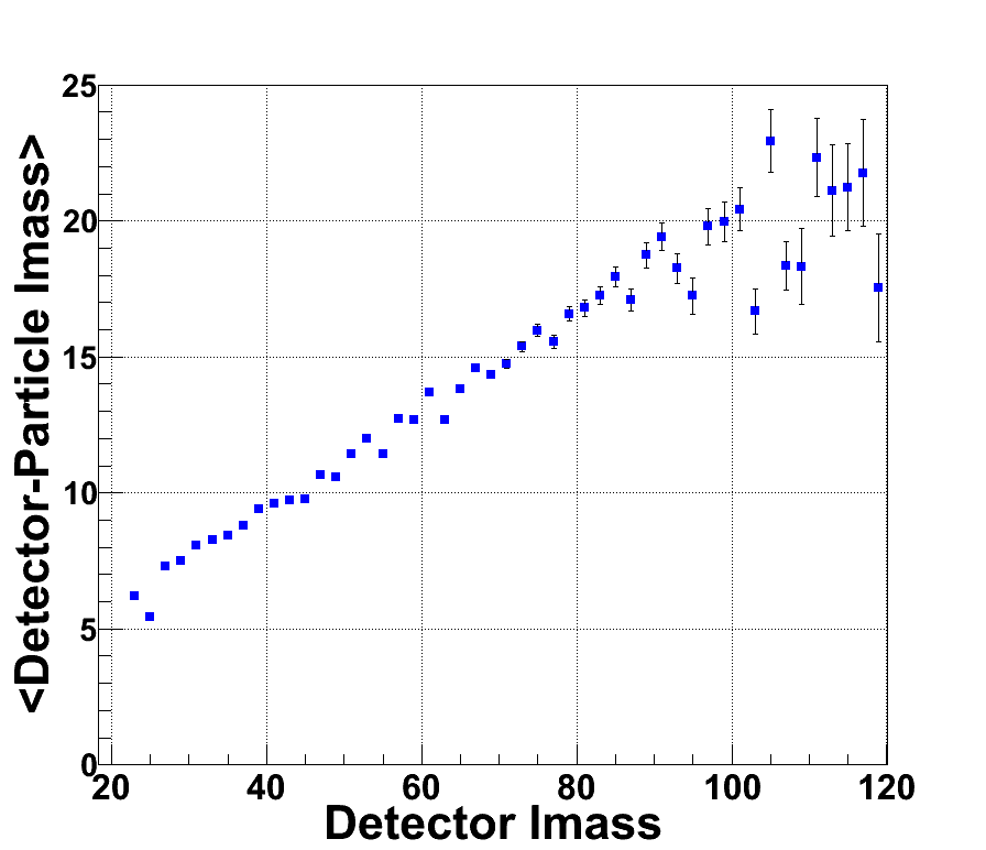
                               Figure 4: Average difference of Detector and Particle Level Invariant Mass as a function of Detector Invariant Mass

The ultimate objective is to determine the origin of the unexpected Imass distribution shown in Figure 3. Therefore, we start by examing the pT3, pT4, ∆eta, and ∆phi at the particle and detector levels. You can see from the following 6 plots the ∆eta and ∆phi at the detector level and particle level have a 1-1 ratio as expected. The main differences lies in the pT distributions. We observe that the particle level jet pT is larger than the detector level jet pT.  If we use the mean values of the following four plots to determine the invariant mass (ignoring jet mass) at the detector and particle level, we will find that the Imass of ~41GeV at the detector level correspond to an Imass of ~50GeV  at the particle level.  This is approxiamely what we arte seeing in Figure 3. Therefore, we can clearly pinpoint that the cause invariant mass distribution observed is due to the jet pT distributions.

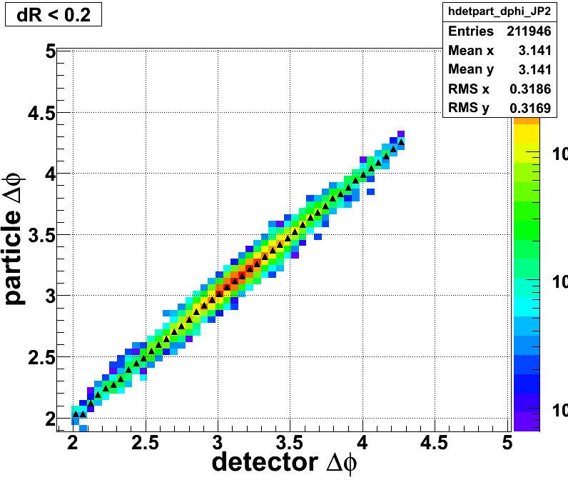
                           Figure 5: The particle level ∆phi as a function of detector level ∆phi (JP2)

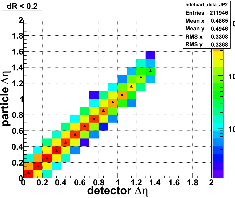
                                     Figure 6: The particle level ∆eta as a function of detector level ∆eta (JP2)

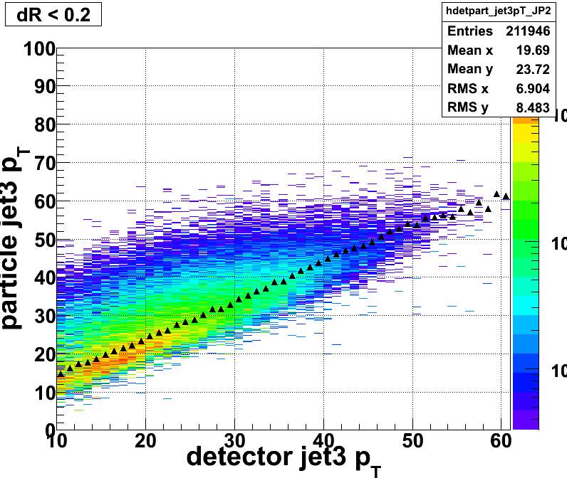
                                    Figure 7: The particle level jet3 pT as a function of detector level jet3 pT (JP2)

                        Figure 8: Average difference of Detector and Particle Level jet3 pT as a function of  Detector jet3 pT

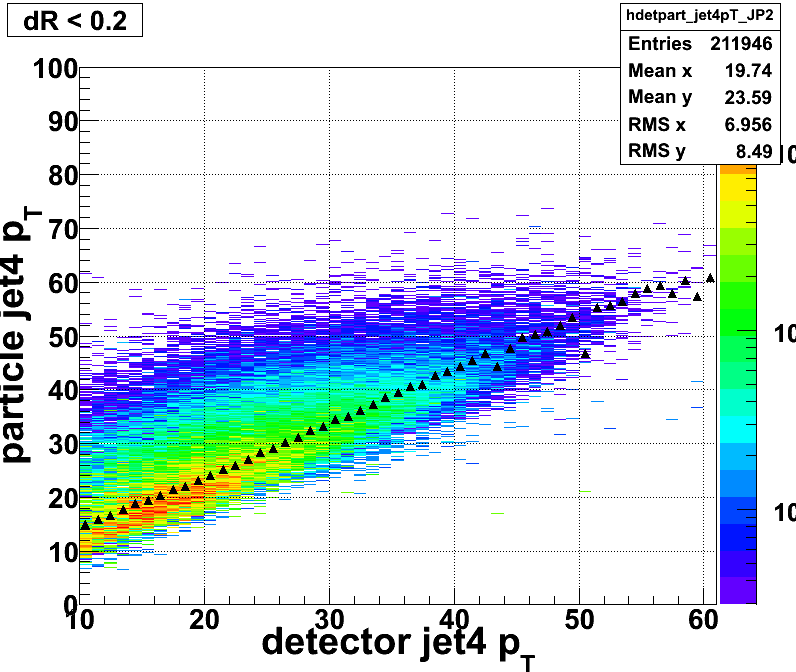
                                    Figure 9: The particle level jet4 pT as a function of detector level jet4 pT(JP2)


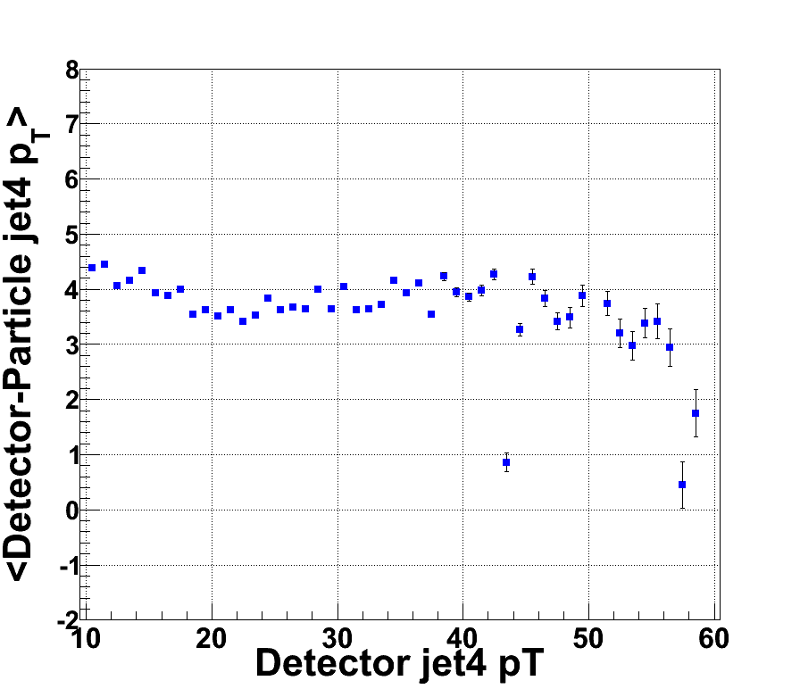
                    Figure 10: Average difference of Detector and Particle Level jet4 pT as a function of  Detector jet4 pT

This correlation is different from Pibero's 2009 pp200 Inclusive Jet pT shift Studies. The correct distributions appear to follow the same direction but we aren't sure if the magnitude is correct.


We next looked at the detector level dijet quantities as a function of the Imass and then look same plots for the particle level.

                                               Figure 11: The detetector level vs the particle level jet pT spectrum (JP2)

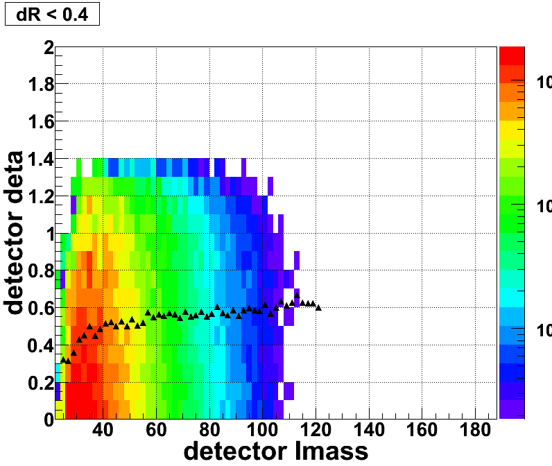
                           Figure 12: The detector level ∆eta as a function of Invariant Mass (JP2)

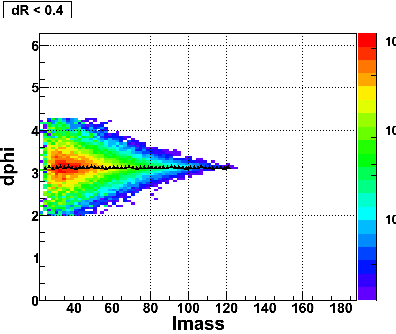
                       Figure 13: The detector level ∆phi as function of the detector level Invariant mass (JP2)

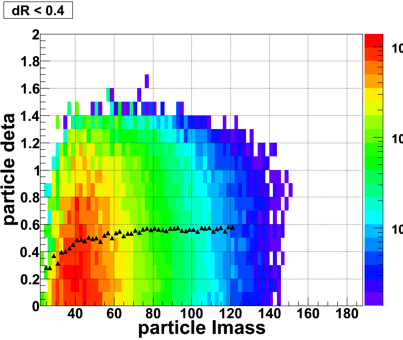
                           Figure 14: The particle level ∆eta as a function of Invariant Mass (JP2)

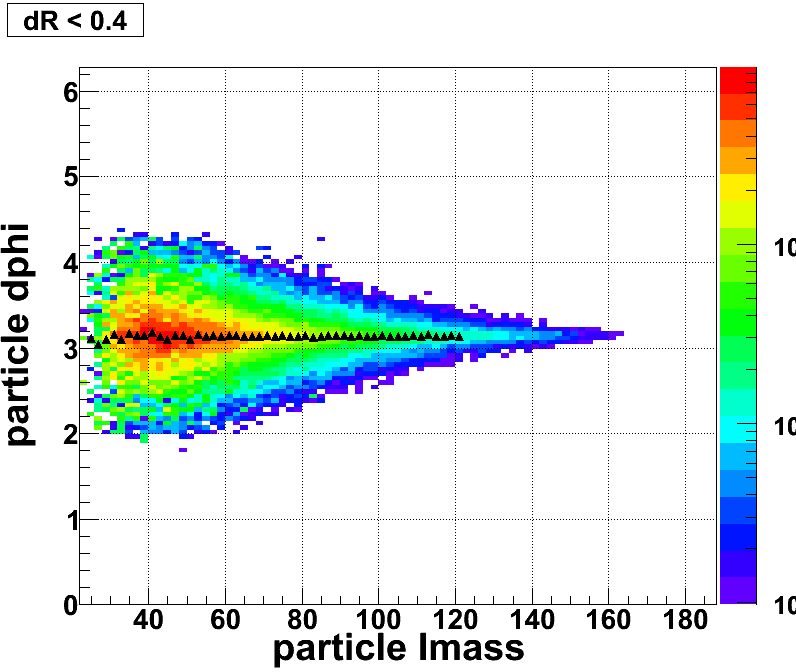
                           Figure 15: The particle level ∆phi as a function of Invariant Mass (JP2)



The ratio of the particle (from .pythia.root) dijets with only the assymetric pT, jet eta, and dphi cut  vs  particle dijets that match with a detector dijet.

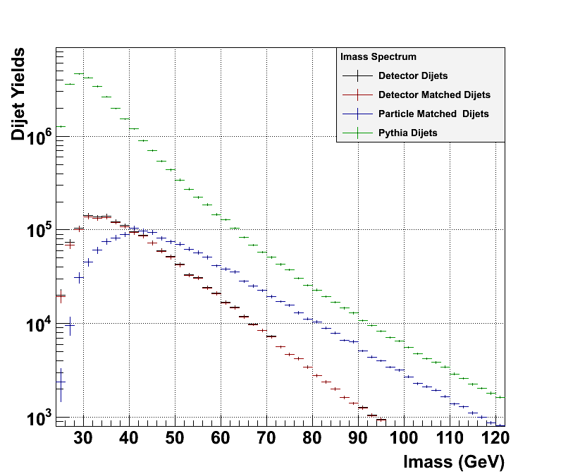
At the previous analysis meeting I gave a talk about the Fake Jet Inefficiencies (R1) using a dR < 0.2 cut. From this we found that we were seeing ~5% unmatched jets (or "fake" dijets) in our sample at the lowest invariant sample. However, to further examine the effect of the dR cut we loosened it to dR < 0.5 as done for the pp200 inclusive jet analysis. You can see the effects of this in the following two plots:

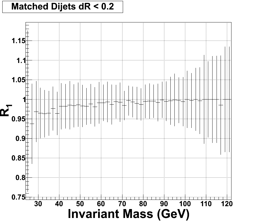
Ignore the error bars above. They are just the sum of the relative errors of the numerator and denominator of the effieciency, which are obviously wrong since the errors very much correlated. The errors of the following plot with the loosened dR cut have the appropriate error calculations.

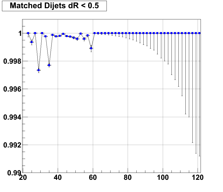
It appears that by loosening the dR cut to 0.5, jets that were once labeled as "fake" are now have a particle jet matched to it. Also, it appears that an overwhelming majority of fake jets are now gone, greater than 99% of the jets are matched. This leads us to conclude that we don't need to account for this infficiency, and we will remove R1 from the equation.