- genevb's home page
- Posts
- 2025
- 2024
- 2023
- 2022
- September (1)
- 2021
- 2020
- 2019
- 2018
- 2017
- December (1)
- October (3)
- September (1)
- August (1)
- July (2)
- June (2)
- April (2)
- March (2)
- February (1)
- 2016
- November (2)
- September (1)
- August (2)
- July (1)
- June (2)
- May (2)
- April (1)
- March (5)
- February (2)
- January (1)
- 2015
- December (1)
- October (1)
- September (2)
- June (1)
- May (2)
- April (2)
- March (3)
- February (1)
- January (3)
- 2014
- 2013
- 2012
- 2011
- January (3)
- 2010
- February (4)
- 2009
- 2008
- 2005
- October (1)
- My blog
- Post new blog entry
- All blogs
Revisiting the wrong TOF THUB clock
Updated on Tue, 2025-04-29 13:28. Originally created by genevb on 2025-04-07 11:04.
The issue was that a different (internal THUB) 40 MHz clock was used for 1/4th of TOF (including VPD west, but not east) than the rest of the system. Usually all are on one common external clock, and this was realized and fixed after run 24162048 shortly after 9pm on June 11, 2023. Geary described the issue with some additional details in an email sent to the MTDTOF mailing list. Zhangbu suggested that the drift in timing could be measured using the difference between TPC and VPD vertex z positions. And I suggested a method of correcting for this in a blog post: Correct timing error for wrong TOF THUB clock.
T0err = 2*(VtxZTPC - VtxZVPD) / c
where c is the speed of light in [cm/ns].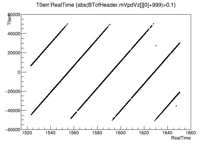
Both plots show the drifting (rising) timing error as real time elapses. The events in the st_physics_adc file are more sparse, making the bands less distinct, but it spans a larger duration of real time. I suspect the two outliers in the left plot are the result of events with low VPD multiplicity such that a random VPD hit alters its time calculation, or the use of a pile-up vertex from the TPC, and should be excluded.
Here are some quick observations...
Another point to discuss from the above plots is that there are clearly two bands at any given real time. I believe this can be understood to be due to the arrival of particles at the VPD detectors before or after rollovers of the time counters. As an illustrative example, one can imagine a moment in time when the arrival of particles at the east VPD is somewhere around halfway through the count up to 51.2 μs (51200 ns), perhaps at about 25.6 μs. And at that moment, if the counter for the west VPD is close to 180° out of phase, close to its moment of rollover back to zero, then the west VPD hits may have a time either very high (just below 51.2 μs) or very low (just above 0). So the VPD east-west time difference can be ±25.6 μs (near one or the other, not between somewhere).
Additional evidence to support this explanation comes from looking at the first plot above as a lego plot, which provides the approximate probability of being in one band vs. the other at any given real time. We see that the probability to be in any one band peaks when the time error is near zero, corresponding to the two counters being in phase. Being in phase is similar to normal operation of both VPDs using a common counter, and is a desirable situation because the probability of seeing only a single band is nearly 1.0 (i.e. the chance that some VPD hits arrive before a counter rollover, and some after a counter rollover is very close to zero, though not exactly zero). The probability to be in either of two bands equalizes (i.e. both bands are on their peaks' respective shoulders) half way between these peaks, when the counters are 180° out of phase.
But to be clear, there is no single "correct" band: both are equally legitimate, and all of it must be corrected to recover the data.
CorrectedT0err = T0err - (51200 ns) * (fmod(RealTime,X)/X) + (51200 ns) * Y
where X is the periodicity in seconds, Y is an integer for the band, and effectively the value of (51200 ns / X) is the timing drift rate in [ns/s]. I manually tuned the value of X to within approximately ±0.01 seconds to make the resulting plot of CorrectedT0err vs. real time as flat as I could for the two MuDsts noted earlier, and here is what I observe:
Run 24161026: X = 36.74 seconds, drift rate = 1394 ns/s = 1.394 μs/s

Run 24140017: X = 37.99 seconds, drift rate = 1348 ns/s = 1.348 μs/s

[small notes: (1) when making these plots, I found that if I had the 51200 ns value incorrect, e.g 52100 ns, it showed up clearly as discontinuities at the clock rollover points in real time, so the smoothness we see here is also further confirmation of the correctness of that 51200 ns value; (2) I made these two particular plots using twice the period as visible in the plots' titles, but that still worked, and I have it correct in the text outside the plots, and I got it corrected for subsequent plots below]
There are a couple striking things to observe here:
A quick order-of-magnitude check to consider is whether a poorly calibrated TPC (e.g. preliminary drift velocities) could contribute. But here we are speaking about a 100 ns shift in the VPD's time, not the TPC's. The TPC vertex position would need be shifted by 15 meters in the formula for T0err for the VPD to result in a 100 ns shift, so this is not TPC-induced.
I'll also add one more observation: in the corrected T0err plot for run 24161026, there is a small set of data points that appear to be shifted upwards by roughly 40 ns. It would be good to understand the cause...perhaps something like a single outlier VPD tube being included?
I automated my above "by eye" method of flattening T0err through subtracting a linearly varying offset by finding a minimum for the RMS in CorrectedT0err, with some basic attempt at automated outlier rejection for the random outliers. I have attached the code to this Drupal page. I then applied this to 784 st_physics_adc files from FastOffline for runs 24140005-24142018 to see what I could learn...
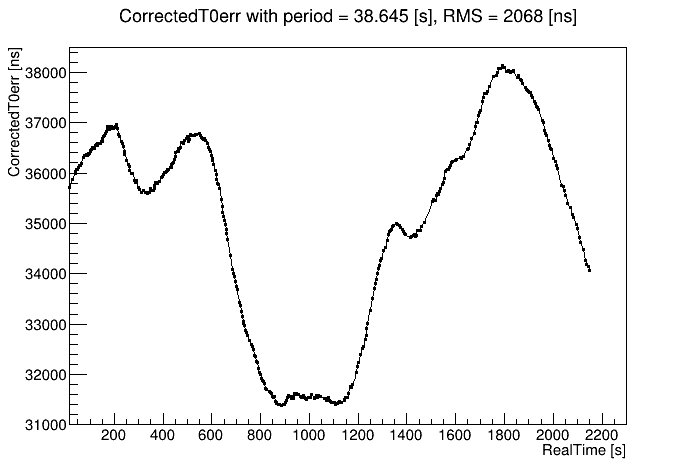
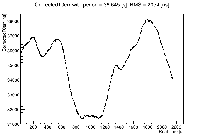
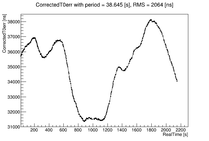
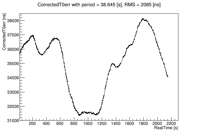
First, there were runs with multiple st_physics_adc files written concurrently. This allowed me to see how reproducible the observed variations were from sampling different events within the same run. Here I show correctedT0err vs. real time for 4 different files (of 20 that all look almost identical!) from run 24140080. The consistency from one sample to the next is impressive!
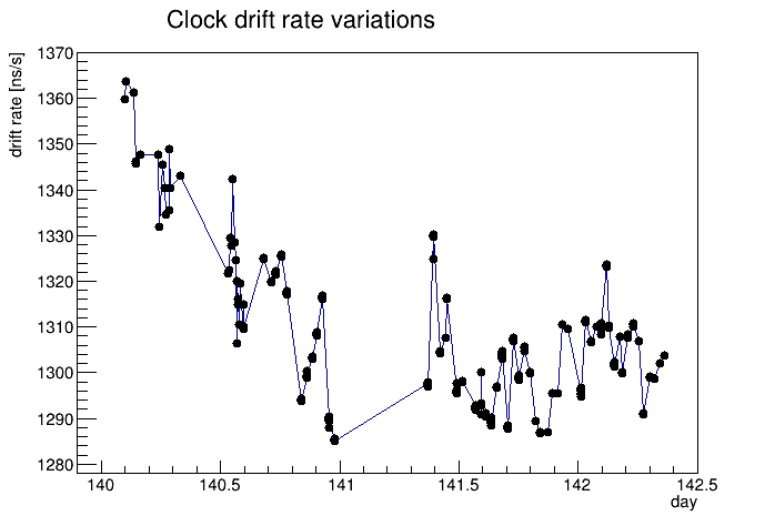
Each and every run shows variations like this that to my eye have no clear time-wise nor run-wise patterns, fluctuating wildly. And this is on top of a different period (or drift rate, which equals 51200 ns / period) used to flatten each run's plot of correctedT0err as much as possible. Below is the distribution of those drift rates used to flatten the plots vs. day number in 2023 (these were runs from days 140-142), showing how the overall drift rate slowed down during that time, but was continuously fluctuating.
[small note: many of the runs had multiple st_physics_adc files, so many of the points in the below graph actually consist of multiple overlapping markers because the automated fitting found consistent results for the multiple files, as demonstrated in the 4 example plots just above]
Some quantifications in terms of the clock rates:
The same information can be presented in a difference way, as the intercept and period can be used to determine a "phase" = period * (intercept/51200) = intercept / drift rate, which is essentially the time before real time = 0 at which the band crossed T0err = 0. Another way to say this is the time between the two THUB clocks being perfectly in phase with each other, and real time = 0. Since the periods only vary modestly, these phases are clustered like the intercepts are, curiously preferring phases of 25-30 seconds:
I concluded earlier in this post that real time = 0 is the time at which any particular run begins (i.e. the bunch count which I'm reading starts at 0 for each run), and I expected no correlation between the phase of T0err and the start of the run. Perhaps the two THUB clocks are reset at the start of each run as well, placing them in a particular phase with respect to each other at each reset? If so, that phase cannot be 0, as such a reset cannot magically be made retroactively 25-30 seconds before a run starts.
One additional thing I checked was whether this phase correlated with the quantity (firstEventTime - runStartTime), as this is something that can vary. It turns out that for the 84 runs I used in this study from days 140-142, all but 8 had (firstEventTime - runStartTime) = 9 seconds, with these 8 ranging from 1-22 seconds. Regardless, there is enough variation to see that no correlation is apparent.
A summarizing presentation for the 2025-04-30 TOF/MTD meeting is attached to this Drupal post as well.
-Gene
Introduction
This is a follow-up to some discussions in 2023, motivated by my observation in attempting to calibrate TPC SpaceCharge for Run 23 AuAu200 that I was unable to get agreement between TPC and VPD vertex z positions for data in early Run 23.The issue was that a different (internal THUB) 40 MHz clock was used for 1/4th of TOF (including VPD west, but not east) than the rest of the system. Usually all are on one common external clock, and this was realized and fixed after run 24162048 shortly after 9pm on June 11, 2023. Geary described the issue with some additional details in an email sent to the MTDTOF mailing list. Zhangbu suggested that the drift in timing could be measured using the difference between TPC and VPD vertex z positions. And I suggested a method of correcting for this in a blog post: Correct timing error for wrong TOF THUB clock.
Measurement
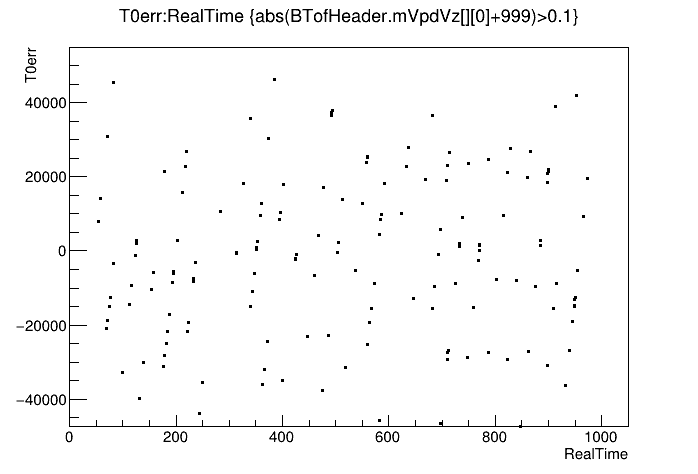
I realized that it is simple to attempt to generate the expected sawtooth plot from the MuDsts. Here are some example plots from an st_physics MuDst file (st_physics_24161026_raw_0500029.MuDst.root), and an st_physics_adc MuDst file (st_physics_adc_24140017_raw_0000007.MuDst.root) of the timing error T0err [ns] vs. real time [s].T0err = 2*(VtxZTPC - VtxZVPD) / c
where c is the speed of light in [cm/ns].
MuDst->SetAlias("T0err","2*(MuEvent.mEventSummary.mPrimaryVertexPos.mX3-BTofHeader.mVpdVz[][0])/29.98");
MuDst->SetAlias("RealTime","(MuEvent.mEventInfo.mBunchCrossingNumber[][0]
+MuEvent.mEventInfo.mBunchCrossingNumber[][1]*pow(2,32))/9383180.0")
TCut VpdFoundVtx = "abs(BTofHeader.mVpdVz[][0]+999)>0.1";
MuDst->SetMarkerStyle(7);
MuDst->Draw("T0err:RealTime",VpdFoundVtx);
Both plots show the drifting (rising) timing error as real time elapses. The events in the st_physics_adc file are more sparse, making the bands less distinct, but it spans a larger duration of real time. I suspect the two outliers in the left plot are the result of events with low VPD multiplicity such that a random VPD hit alters its time calculation, or the use of a pile-up vertex from the TPC, and should be excluded.
Here are some quick observations...
- The bunch crossing numbers appear to reset for each run, not each fill. This implies that the phase for the correction must be determined run-by-run, not fill-by-fill.
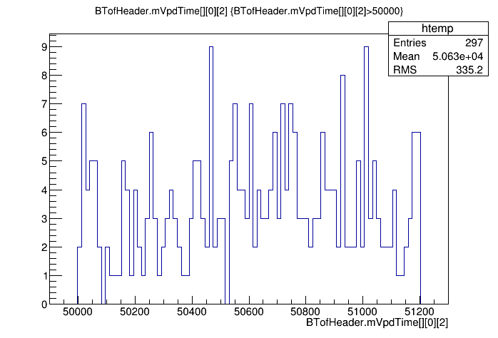
- The maximum VPD time shows a rather clean cut at 51200 ns (51.2 μs), which is a small surprise as we were expecting it to be twice that, at 102.4 μs. This can be seen graphically rather easily from the MuDst as well, though I confirmed the values with print statements inside StVpdCalibMaker.
- UPDATE: I believe I tracked this down to the HPTDC manual (pages 24 & 67) indicating that the most-significant-bit is dropped at readout when using the very high precision mode.
MuDst->Draw("BTofHeader.mVpdTime[][0][2]","BTofHeader.mVpdTime[][0][2]>50000")
Another point to discuss from the above plots is that there are clearly two bands at any given real time. I believe this can be understood to be due to the arrival of particles at the VPD detectors before or after rollovers of the time counters. As an illustrative example, one can imagine a moment in time when the arrival of particles at the east VPD is somewhere around halfway through the count up to 51.2 μs (51200 ns), perhaps at about 25.6 μs. And at that moment, if the counter for the west VPD is close to 180° out of phase, close to its moment of rollover back to zero, then the west VPD hits may have a time either very high (just below 51.2 μs) or very low (just above 0). So the VPD east-west time difference can be ±25.6 μs (near one or the other, not between somewhere).
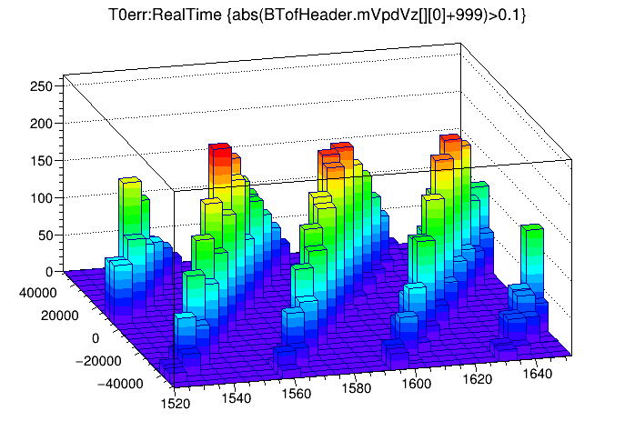
Additional evidence to support this explanation comes from looking at the first plot above as a lego plot, which provides the approximate probability of being in one band vs. the other at any given real time. We see that the probability to be in any one band peaks when the time error is near zero, corresponding to the two counters being in phase. Being in phase is similar to normal operation of both VPDs using a common counter, and is a desirable situation because the probability of seeing only a single band is nearly 1.0 (i.e. the chance that some VPD hits arrive before a counter rollover, and some after a counter rollover is very close to zero, though not exactly zero). The probability to be in either of two bands equalizes (i.e. both bands are on their peaks' respective shoulders) half way between these peaks, when the counters are 180° out of phase.
But to be clear, there is no single "correct" band: both are equally legitimate, and all of it must be corrected to recover the data.
Correction Attempt
Next, I attempted a "by eye" correction. Ignoring the phase, I can simply try to make the T0err constant at its intercept value by subtracting an offset that varies linearly in real time, and adding a "band-wise" correction:CorrectedT0err = T0err - (51200 ns) * (fmod(RealTime,X)/X) + (51200 ns) * Y
where X is the periodicity in seconds, Y is an integer for the band, and effectively the value of (51200 ns / X) is the timing drift rate in [ns/s]. I manually tuned the value of X to within approximately ±0.01 seconds to make the resulting plot of CorrectedT0err vs. real time as flat as I could for the two MuDsts noted earlier, and here is what I observe:
double X = 36.74; // seconds
MuDst->Draw(Form("T0err-51200*fmod(RealTime,%5.2f)/%5.2f
+51200*(3-int((T0err-51200*fmod(RealTime,%5.2f)/%5.2f)/51200+3))
:RealTime",X,X,X,X),VpdFoundVtx);
Run 24161026: X = 36.74 seconds, drift rate = 1394 ns/s = 1.394 μs/s
Run 24140017: X = 37.99 seconds, drift rate = 1348 ns/s = 1.348 μs/s
[small notes: (1) when making these plots, I found that if I had the 51200 ns value incorrect, e.g 52100 ns, it showed up clearly as discontinuities at the clock rollover points in real time, so the smoothness we see here is also further confirmation of the correctness of that 51200 ns value; (2) I made these two particular plots using twice the period as visible in the plots' titles, but that still worked, and I have it correct in the text outside the plots, and I got it corrected for subsequent plots below]
There are a couple striking things to observe here:
- The two runs have clearly different drift rates (and consequently periods). It isn't a question whether they may be the same within errors: using one's X value for the other leaves a significant drift.
- Even after the correction, there are remaining variations at the O(100 ns) level in the first plot, and O(1500 ns) level in the second plot. These are compatible with each other in the sense that the second plot spans a much larger real time interval, and in some real time intervals similar to the first plot's, it also shows only O(100 ns) variations. The variations are smoothly flowing, as if a clock speed slowly varies.
A quick order-of-magnitude check to consider is whether a poorly calibrated TPC (e.g. preliminary drift velocities) could contribute. But here we are speaking about a 100 ns shift in the VPD's time, not the TPC's. The TPC vertex position would need be shifted by 15 meters in the formula for T0err for the VPD to result in a 100 ns shift, so this is not TPC-induced.
I'll also add one more observation: in the corrected T0err plot for run 24161026, there is a small set of data points that appear to be shifted upwards by roughly 40 ns. It would be good to understand the cause...perhaps something like a single outlier VPD tube being included?
Clock Instability
From my analysis, we don't actually know whether it is the local THUB clock that has an instability, the external clock, or possibly even both. We just see an instability in the difference between the two.I automated my above "by eye" method of flattening T0err through subtracting a linearly varying offset by finding a minimum for the RMS in CorrectedT0err, with some basic attempt at automated outlier rejection for the random outliers. I have attached the code to this Drupal page. I then applied this to 784 st_physics_adc files from FastOffline for runs 24140005-24142018 to see what I could learn...
First, there were runs with multiple st_physics_adc files written concurrently. This allowed me to see how reproducible the observed variations were from sampling different events within the same run. Here I show correctedT0err vs. real time for 4 different files (of 20 that all look almost identical!) from run 24140080. The consistency from one sample to the next is impressive!
Each and every run shows variations like this that to my eye have no clear time-wise nor run-wise patterns, fluctuating wildly. And this is on top of a different period (or drift rate, which equals 51200 ns / period) used to flatten each run's plot of correctedT0err as much as possible. Below is the distribution of those drift rates used to flatten the plots vs. day number in 2023 (these were runs from days 140-142), showing how the overall drift rate slowed down during that time, but was continuously fluctuating.
[small note: many of the runs had multiple st_physics_adc files, so many of the points in the below graph actually consist of multiple overlapping markers because the automated fitting found consistent results for the multiple files, as demonstrated in the 4 example plots just above]
Some quantifications in terms of the clock rates:
- These drift rates are on the order of 1.3 parts per million. That implies a ~50 Hz difference between two 40 MHz clocks in general.
- The variations in drift rate are at the level of at least 1.3 parts per 10 million, so variations at the level of ~5 Hz or more for that ~50 Hz difference during the time the internal THUB clock was used in Run 23.
- A quantification of the variation rate can be gleaned from the above plots for run 24140080, where a ~5500 ns drop in correctedT0err occurs in roughly 300 seconds. That represents about 18 parts per billion, so the 40 MHz clock changed by ~0.75 Hz over a span of ~5 minutes, or ~0.15 Hz/minute.
Intercept and Phase Stability
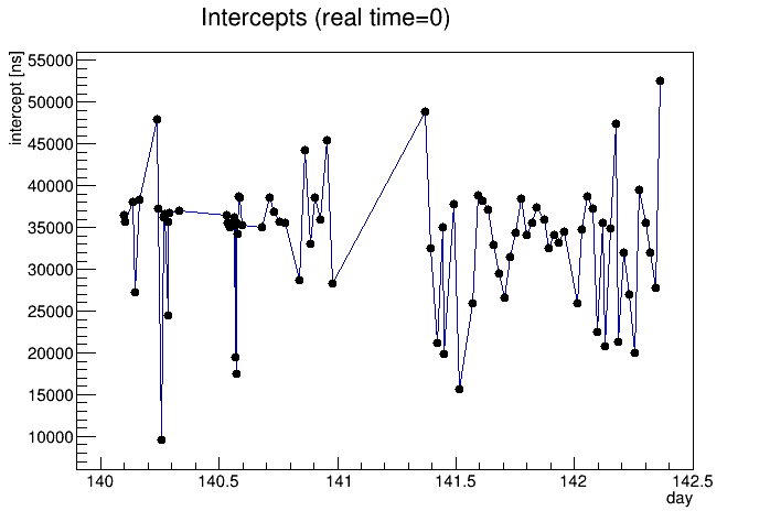
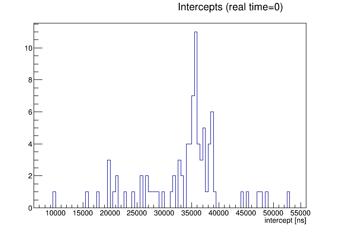
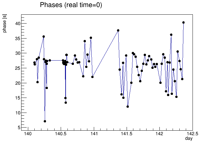
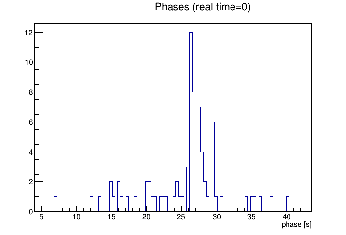
I also noticed something I didn't expect coming out of the automated flattening: I can define the "intercept" as the vertical location the bands cross real time = 0. This comes directly as the mean of my correcedT0err for each run, because I'm subtracting a correction that starts as 0 at real time = 0, so I'm flattening the sawtooth to the value at real time = 0. Here, using just one data point (one st_physics_adc file) per run, is the distribution of intercepts, showing a clear preference for intercepts in the range of 35000-40000 ns:The same information can be presented in a difference way, as the intercept and period can be used to determine a "phase" = period * (intercept/51200) = intercept / drift rate, which is essentially the time before real time = 0 at which the band crossed T0err = 0. Another way to say this is the time between the two THUB clocks being perfectly in phase with each other, and real time = 0. Since the periods only vary modestly, these phases are clustered like the intercepts are, curiously preferring phases of 25-30 seconds:
I concluded earlier in this post that real time = 0 is the time at which any particular run begins (i.e. the bunch count which I'm reading starts at 0 for each run), and I expected no correlation between the phase of T0err and the start of the run. Perhaps the two THUB clocks are reset at the start of each run as well, placing them in a particular phase with respect to each other at each reset? If so, that phase cannot be 0, as such a reset cannot magically be made retroactively 25-30 seconds before a run starts.
One additional thing I checked was whether this phase correlated with the quantity (firstEventTime - runStartTime), as this is something that can vary. It turns out that for the 84 runs I used in this study from days 140-142, all but 8 had (firstEventTime - runStartTime) = 9 seconds, with these 8 ranging from 1-22 seconds. Regardless, there is enough variation to see that no correlation is apparent.
Conclusion
In summary, what I have seen of the clock instabilities so far leads unfortunately to low expectations for being able to sufficiently correct all events' TOF timing errors in this data via functional fits to the time dependence.A summarizing presentation for the 2025-04-30 TOF/MTD meeting is attached to this Drupal post as well.
-Gene
»
- genevb's blog
- Login or register to post comments