- genevb's home page
- Posts
- 2025
- 2024
- 2023
- 2022
- September (1)
- 2021
- 2020
- 2019
- December (1)
- October (4)
- September (2)
- August (6)
- July (1)
- June (2)
- May (4)
- April (2)
- March (3)
- February (3)
- 2018
- 2017
- December (1)
- October (3)
- September (1)
- August (1)
- July (2)
- June (2)
- April (2)
- March (2)
- February (1)
- 2016
- November (2)
- September (1)
- August (2)
- July (1)
- June (2)
- May (2)
- April (1)
- March (5)
- February (2)
- January (1)
- 2015
- December (1)
- October (1)
- September (2)
- June (1)
- May (2)
- April (2)
- March (3)
- February (1)
- January (3)
- 2014
- December (2)
- October (2)
- September (2)
- August (3)
- July (2)
- June (2)
- May (2)
- April (9)
- March (2)
- February (2)
- January (1)
- 2013
- December (5)
- October (3)
- September (3)
- August (1)
- July (1)
- May (4)
- April (4)
- March (7)
- February (1)
- January (2)
- 2012
- December (2)
- November (6)
- October (2)
- September (3)
- August (7)
- July (2)
- June (1)
- May (3)
- April (1)
- March (2)
- February (1)
- 2011
- November (1)
- October (1)
- September (4)
- August (2)
- July (4)
- June (3)
- May (4)
- April (9)
- March (5)
- February (6)
- January (3)
- 2010
- December (3)
- November (6)
- October (3)
- September (1)
- August (5)
- July (1)
- June (4)
- May (1)
- April (2)
- March (2)
- February (4)
- January (2)
- 2009
- November (1)
- October (2)
- September (6)
- August (4)
- July (4)
- June (3)
- May (5)
- April (5)
- March (3)
- February (1)
- 2008
- 2005
- October (1)
- My blog
- Post new blog entry
- All blogs
An update to the recent Run 17 pp510 TPC SpaceCharge calibration
Updated on Thu, 2020-01-16 15:35. Originally created by genevb on 2020-01-13 16:40.
In December 2019, we re-produced 5 fills of data from Run 17 pp510 using a new TPC SpaceCharge calibration. The calibration was done fill-by-fill, using a formula to obtain the fill-by-fill dependence based on the fill-by-fill measurement of the ratio of +/- at high pT (let's call that ratio R). That formula was determined by a simple fit made with 7 directly re-calibrated fills of the SpaceCharge coefficient (other parameters of the SpaceCharge & GridLeak correction were determined from a fit using all 7 fills of data at once to arrive at a single set of values that would be used for all fills; i.e. only the SpaceCharge coefficient parameter is allowed to vary fill-by-fill). However, a consideration was overlooked in deciding the form of that formula: the value of R depends on the error in the original SpaceCharge from 2017. But because the new 2019 SpaceCharge calibration has a slightly different luminosity dependence, the conversion of R into a new SpaceCharge coefficient must also account for how different the 2017 and 2019 SpaceCharge corrections are at any given luminosity. One could write this as:
December 2019 correction: SCfill = func(Rfill)
early-January-2020 correction: SCfill = func(Rfill,<Lumi>fill)
...and we specifically use the luminosity dependence straight from the global SpaceCharge calibration functions...
sc = SC * (lumi - SO)
sc_old = 6.845e-8 * (zdcenk - 61030)
sc_new = SC_new * (zdcwnk + 15170)
func(R) = sc_new - sc_old <=== we can assume some form for func(R) that empirically matches the results of the re-calibration of sc_new for a few fills
sc_new = func(R) + sc_old
...thus...
SCfill = (func(Rfill) + 6.845e-8 * (<zdcenk>fill - 61030)) / (<zdcwnk>fill + 15170)
The math to consider this was accounted as above to obtain a new func(R) determined by fitting (sc_old - sc_new) vs. R for 7 re-calibrated fills (using <zdcenk> and <zdcwnk> for those fills). To truly see if this is better, we should probably reproduce the data yet again.
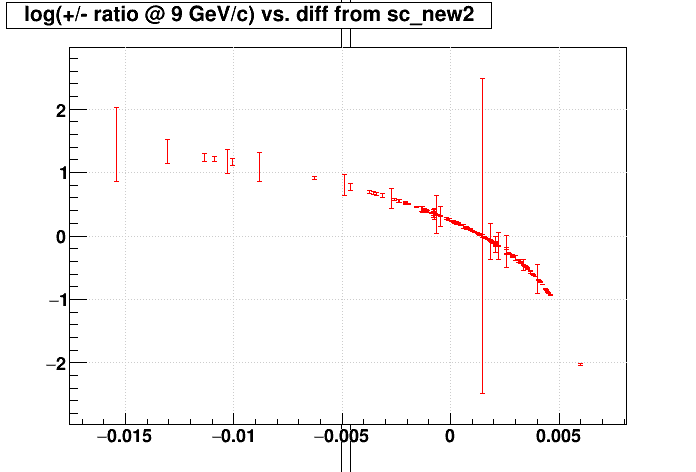
However, in the interim, there is another way to learn about whether the new early-January-2020 SpaceCharge coefficients will improve things. Jae presented in December the high pT +/- ratios using the 2017 and 2019 calibrations, with fit parameters that allowed a determination of R. Again, the value of R should depend monotonically on the error in the SpaceCharge correction that was used, so we can plot R versus that error under two possible assumptions: (1) the 2019 SpaceCharge calibration is the truth, and (2) the early-January-2020 SpaceCharge calibration is the truth.
In the below plots, sc_new1 refers to using the 2019 calibration as the truth, while sc_new2 refers to the early-January-2020 calibration. The vertical axis is log(R), and the horizontal axis is the SpaceCharge used minus what is postulated to be the true SpaceCharge. Instead of focusing on specific values, I plot the data as its error bar range using the errors reported by Jae (although I think this is an overestimate of the error on the ratio). Black points are the data from the original physics production that used the 2017 calibration, while red points are for the December 2019 production (note that in this production, sc_new1 was used, so assuming it is the truth puts all the data points at 0 on the horizontal axis of the left plot, and I artificially moved them a little bit away from each other so that they could be distinctly seen).
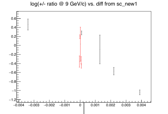
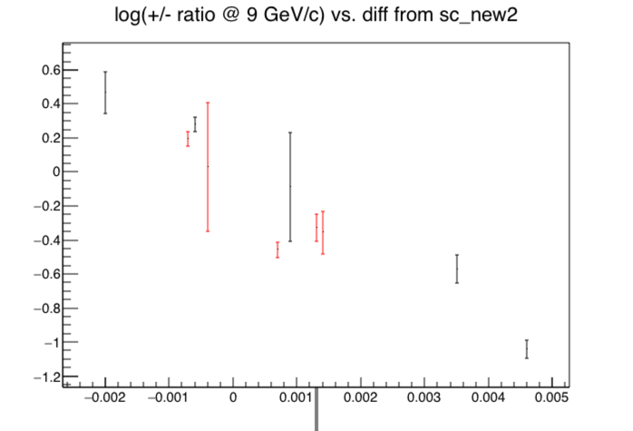
Does the right plot show a more monotonic dependence? It isn't perfect, but Yes! There are really only 1 or 2 data points that are more than one standard deviation away from a simple curve (or line) through all 10 data points. The plot on the left would have 5 such data points. Matt Posik has some possible minor tweaks to the formula we use for the dependence on R, which we will try (before committing to a physics re-production) to see if we can achieve even better monotonicity, but we expect things will change very little from what is already observed.
-Gene
____________________
UPDATE 2020-01-14:
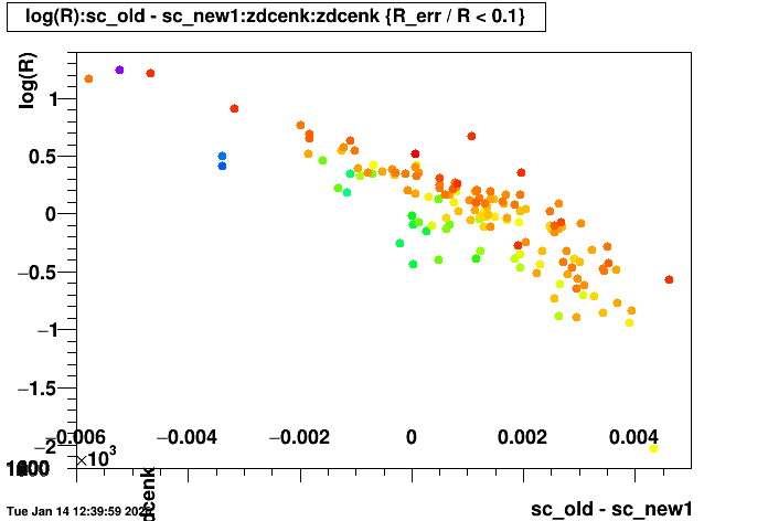
I realized I had what I needed to make the black data in the above plots vs. all fills from the original Run 17 pp510 physics production (158 fills). First, a plot to show the stratification in the plot of log(R) vs difference from sc_new1 with one measure of the mean luminosity (shown via color) for each fill, which makes it clear that a luminosity dependence remained that would not be accounted when using sc_new1 for correcting the data. For this plot, since I couldn't show error bars, I excluded fills which had a large error on R (due to low statistics in that fill).
Now, here are the plots using sc_new1 and sc_new2 for all 158 fills with their error bars, keeping plot axes constant between the two plots:
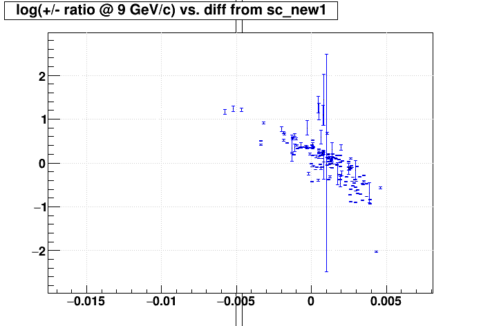
The difference is striking, but the data now all lie on one curve that is determined by the func(R) that we found for the dependence of (sc_old - sc_new) on R, so it is not actually a surprise that the curve is so perfect.
To reiterate: this is a statement that we can find a functional form for calculating SpaceCharge (using only 7 fills) that should correct for much of the luminosity dependence seen in R from that original physics production. It remains to be demonstrated that using the new SpaceCharge calibration brings all the ratios to a single, as-yet-not-determined, physical value.
Yay!
-Gene
____________
UPDATE 2020-01-15:
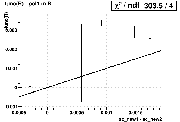
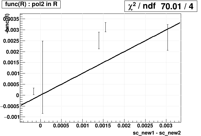
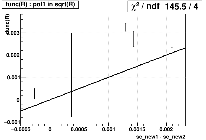
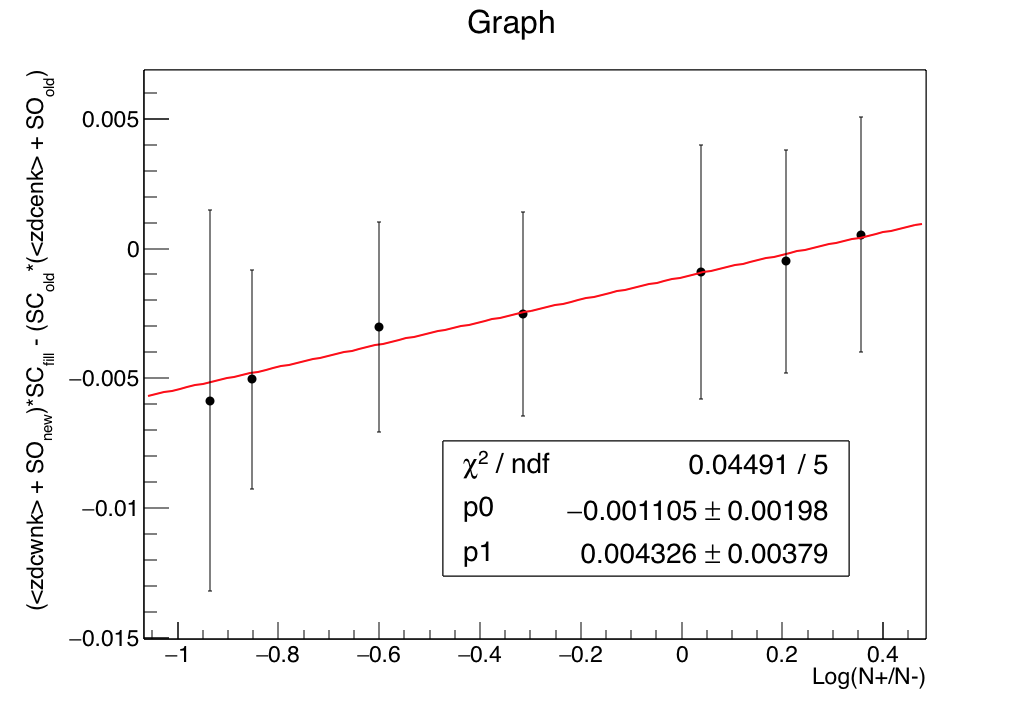
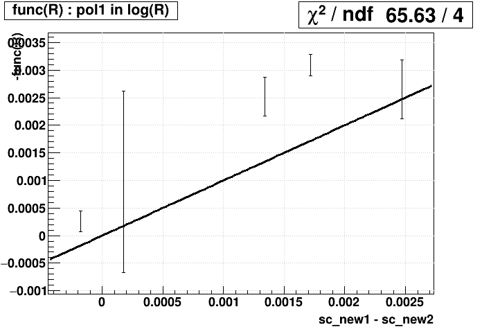
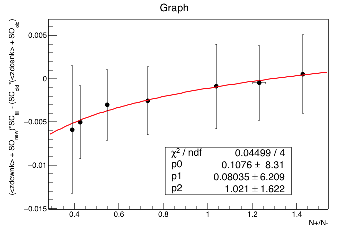
An open question remains: what is the best choice for func(R). To decide this, we have two metrics: (1) goodness-of-fit (Χ2/dof) for func(R) on the plot of (sc_new2 - sc_old) vs. Rold, and (2) goodness-of-fit for func(Rnew1) = sc_new2 - sc_new1, or identically -func(Rnew1) = sc_new1 - sc_new2, where the subscripts "old" and "new1" refer to the SpaceCharge calibration used in producing the data from which that R was measured (i.e. the original physics production, or the December 5-fill sample respectively). These are presented below for candidate functions:
(Tiny sidenote: while the plots on the right show 4 degrees of freedom, it's actually 5; to let ROOT fit the straight line y=x to just show me the Χ2, it required I have at least one fit parameter, so I fit y=x+0*p0 and then just didn't print p0.)
A pol1 in log(R), the functional result of exponential pT distributions, is slightly better than the functional result of hard pT distributions as the top two candidates based on Χ2/dof for both columns. Note also that Jae found exponentials to be a good match in fitting the individual + and - pT distributions. So we will proceed with the pol1 in log(R) function.
-Gene
December 2019 correction: SCfill = func(Rfill)
early-January-2020 correction: SCfill = func(Rfill,<Lumi>fill)
...and we specifically use the luminosity dependence straight from the global SpaceCharge calibration functions...
sc = SC * (lumi - SO)
sc_old = 6.845e-8 * (zdcenk - 61030)
sc_new = SC_new * (zdcwnk + 15170)
func(R) = sc_new - sc_old <=== we can assume some form for func(R) that empirically matches the results of the re-calibration of sc_new for a few fills
sc_new = func(R) + sc_old
...thus...
SCfill = (func(Rfill) + 6.845e-8 * (<zdcenk>fill - 61030)) / (<zdcwnk>fill + 15170)
The math to consider this was accounted as above to obtain a new func(R) determined by fitting (sc_old - sc_new) vs. R for 7 re-calibrated fills (using <zdcenk> and <zdcwnk> for those fills). To truly see if this is better, we should probably reproduce the data yet again.
However, in the interim, there is another way to learn about whether the new early-January-2020 SpaceCharge coefficients will improve things. Jae presented in December the high pT +/- ratios using the 2017 and 2019 calibrations, with fit parameters that allowed a determination of R. Again, the value of R should depend monotonically on the error in the SpaceCharge correction that was used, so we can plot R versus that error under two possible assumptions: (1) the 2019 SpaceCharge calibration is the truth, and (2) the early-January-2020 SpaceCharge calibration is the truth.
In the below plots, sc_new1 refers to using the 2019 calibration as the truth, while sc_new2 refers to the early-January-2020 calibration. The vertical axis is log(R), and the horizontal axis is the SpaceCharge used minus what is postulated to be the true SpaceCharge. Instead of focusing on specific values, I plot the data as its error bar range using the errors reported by Jae (although I think this is an overestimate of the error on the ratio). Black points are the data from the original physics production that used the 2017 calibration, while red points are for the December 2019 production (note that in this production, sc_new1 was used, so assuming it is the truth puts all the data points at 0 on the horizontal axis of the left plot, and I artificially moved them a little bit away from each other so that they could be distinctly seen).
Does the right plot show a more monotonic dependence? It isn't perfect, but Yes! There are really only 1 or 2 data points that are more than one standard deviation away from a simple curve (or line) through all 10 data points. The plot on the left would have 5 such data points. Matt Posik has some possible minor tweaks to the formula we use for the dependence on R, which we will try (before committing to a physics re-production) to see if we can achieve even better monotonicity, but we expect things will change very little from what is already observed.
-Gene
____________________
UPDATE 2020-01-14:
I realized I had what I needed to make the black data in the above plots vs. all fills from the original Run 17 pp510 physics production (158 fills). First, a plot to show the stratification in the plot of log(R) vs difference from sc_new1 with one measure of the mean luminosity (shown via color) for each fill, which makes it clear that a luminosity dependence remained that would not be accounted when using sc_new1 for correcting the data. For this plot, since I couldn't show error bars, I excluded fills which had a large error on R (due to low statistics in that fill).
Now, here are the plots using sc_new1 and sc_new2 for all 158 fills with their error bars, keeping plot axes constant between the two plots:
The difference is striking, but the data now all lie on one curve that is determined by the func(R) that we found for the dependence of (sc_old - sc_new) on R, so it is not actually a surprise that the curve is so perfect.
To reiterate: this is a statement that we can find a functional form for calculating SpaceCharge (using only 7 fills) that should correct for much of the luminosity dependence seen in R from that original physics production. It remains to be demonstrated that using the new SpaceCharge calibration brings all the ratios to a single, as-yet-not-determined, physical value.
Yay!
-Gene
____________
UPDATE 2020-01-15:
An open question remains: what is the best choice for func(R). To decide this, we have two metrics: (1) goodness-of-fit (Χ2/dof) for func(R) on the plot of (sc_new2 - sc_old) vs. Rold, and (2) goodness-of-fit for func(Rnew1) = sc_new2 - sc_new1, or identically -func(Rnew1) = sc_new1 - sc_new2, where the subscripts "old" and "new1" refer to the SpaceCharge calibration used in producing the data from which that R was measured (i.e. the original physics production, or the December 5-fill sample respectively). These are presented below for candidate functions:
(Tiny sidenote: while the plots on the right show 4 degrees of freedom, it's actually 5; to let ROOT fit the straight line y=x to just show me the Χ2, it required I have at least one fit parameter, so I fit y=x+0*p0 and then just didn't print p0.)
| Candidate func(R) | (sc_new2 - sc_old) vs. Rold | -func(Rnew1) vs. sc_new1 - sc_new2 |
|---|---|---|
| pol1 in R | 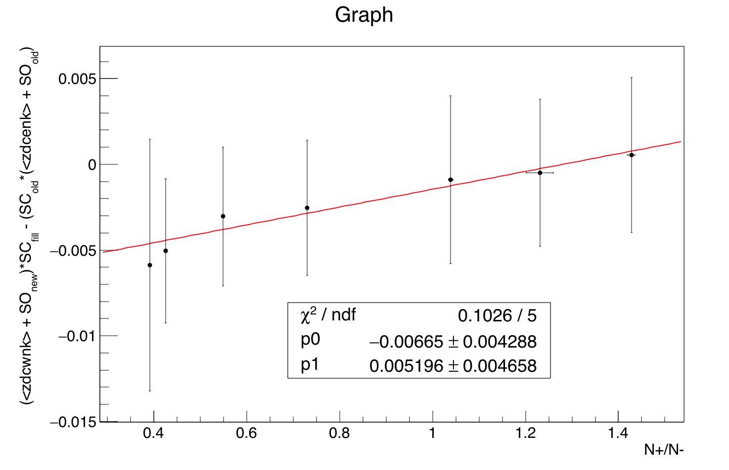 |
 |
| pol2 in R | 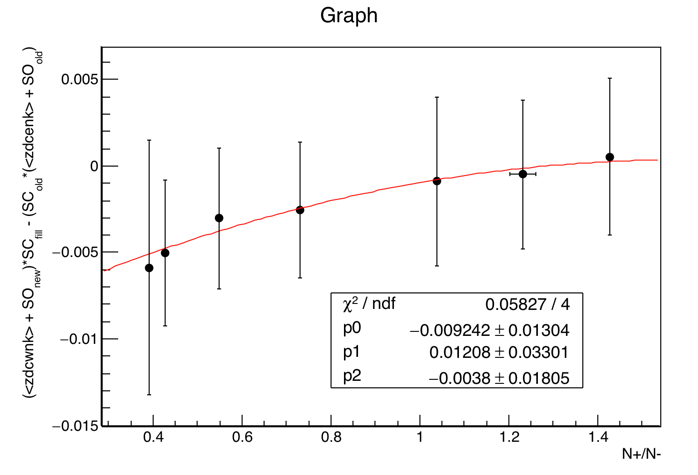 |
 |
| pol1 in sqrt(R) | 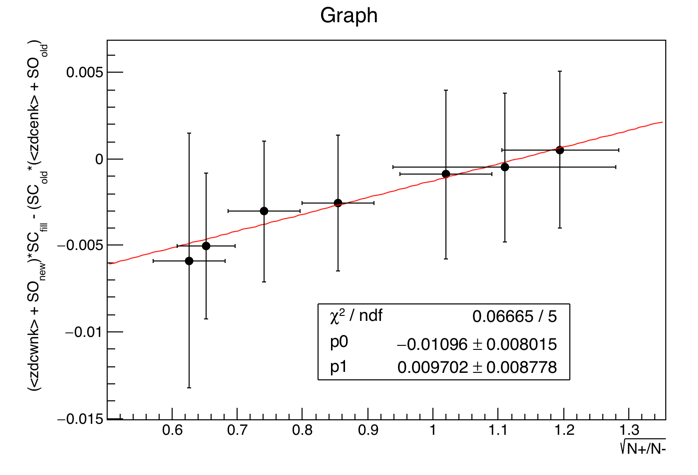 |
 |
| exponential pT spectrum: yield = C * exp(-pT/T) combined with δpT = A * q * pT2 leads to... pol1 in log(R) |
 |
 |
| hard pT spectrum: yield = C * [1 + (pT/p0)]-n combined with δpT = A * q * pT2 leads to... B * (RD - E)/(RD + E) |
 |
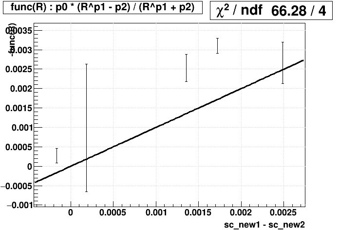 |
A pol1 in log(R), the functional result of exponential pT distributions, is slightly better than the functional result of hard pT distributions as the top two candidates based on Χ2/dof for both columns. Note also that Jae found exponentials to be a good match in fitting the individual + and - pT distributions. So we will proceed with the pol1 in log(R) function.
-Gene
»
- genevb's blog
- Login or register to post comments