A further comparison of the EEMC Tower data from 2006 with the first pass 2009 data since the last blog entry.  Ratios were calculated of each tower gain from the first-pass data to the 2006 final gains.  A histogram of these ratios, ignoring known problematic fits to certain towers, is shown below:

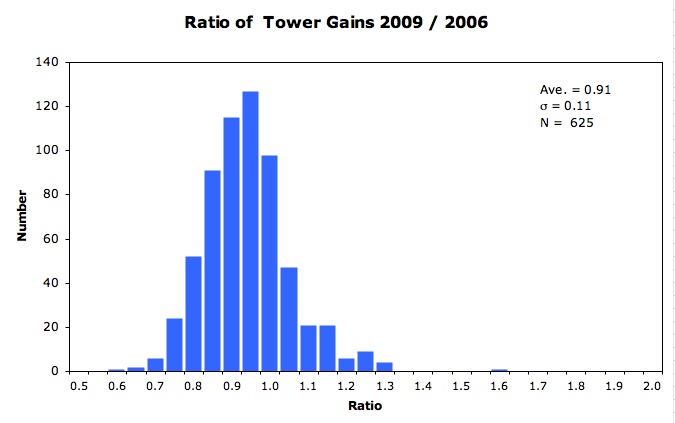
Fig. 1.  Histogram of the ratio of ech tower gain from the first pass 2009 data to the 2006 data.

The average peak of the ratios is located at 0.91, or with the 2009 data about 10% below the 2006 data.  This coincides with an observation that the 2009 gains from the first pass appear to be low by about 10%. 

   The ideal gains, or gains expected from a particle traversing a given tower and depositing 60 GeV of transverse energy, were calculated for each tower.  These ideal gains were then compared to the 2006 data and the first-pass 2009 data.  A histogram was made of the difference in gains (2006 tower gains minus the ideal gains) divided by the ideal and given as a percentage.  This histogram is shown below:

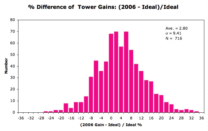
Fig. 2. Histogram of the difference in tower ideal gain from the gain found in the 2006 data divided by the ideal gain.

By rebinning this histogram, shown below, it looks exactly like the plot shown on slide 18 in the 2008 calibration talk by S. Wissink.

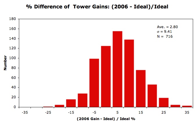
Fig. 3.  Histogram of the difference in tower ideal gain from gain found in 2006 data.  This plot is rebinned from Fig. 2 and compares with the plot from the 2008 talk by S. Wissink.  

   Likewise, a histogram was made of the difference in gains for the 2009 first-pass data, as shown below:

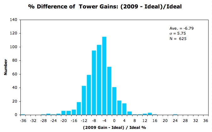
Fig. 4. Histogram of the difference in tower ideal gain from the gain found in the 2009 first-pass data, divided by the ideal gain.

A comparison of figs. 2 and 4 shows that the 2009 data distribution is shifted to the left and has a much narrower spread than the distribution from the 2006 data. 

   Further analysis was made with the first-pass 2009 data for tower sector 9, sub-sector E gains.  Listed in the table below are the ideal gains, which were calculated for each eta bin in that sector, the first-pass gains and errors, and the gains and errors from the convolution method.  Also displayed in Table 1 are comparisons giving the percent differences of the first-pass gains and the convolution-method gains with the ideal gains.  The yellow boxes under the first-pass data in Table 1 show towers with known problems in the fit, namely, the pedestal was included in the fit peak.  The average percent differences from the ideal gains for each of these methods are also shown.  Only the four good points were used in the first-pass average percent difference.  These data are also plotted in Fig. 5 below.

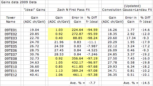
Table 1.  Table of ideal gains, first-pass 2009 gains, and gains from the convolution method on the 2009 data.  Also included are the percent differences of these gains from the ideal gains.  The yellow boxes indicate the towers with known problems in the fit from the first pass of the 2009 data. 

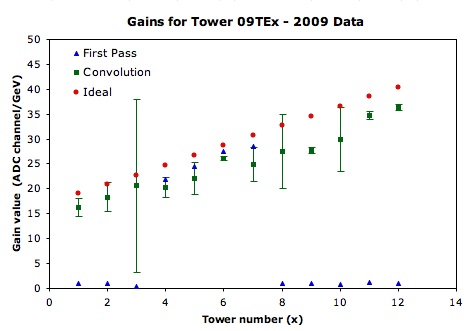
Fig. 5.  Plot of the ideal gains, first-pass gains from 2009 data, and the gains using the convolution method on the 2009 data for towers in sector 9, sub-sector E.  No error bars are included on points from the first-pass method. 

   The tower gains for sector 9, sub-sector E from the 2006 data were added to the data in Table 1 for comparison, and are provided in Table 2.  No gain information was available from 2006 for tower 09TE01.  A column shows the percent difference that each of these gains are from the ideal gains, along with the average percent difference for the entire sub-sector.  It can be seen that several of these gains deviate significantly from the ideal gains.  The average difference of the gains from the ideal gains for this sub-sector is also presented, and is seen to be about 6% above the ideal gain value.  

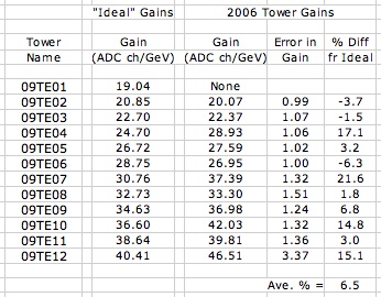
Table 2. Table showing the ideal gains and the final gains and uncertainties using the 2006 data from towers in sector 9, sub-sector E.  The last column lists the percent difference of the gains from the ideal gains. 

These 2006 gains for towers in sector 9, sub-sector E are plotted as a function of eta bin in Fig. 6, along with the data contained in Fig. 5 for comparison.

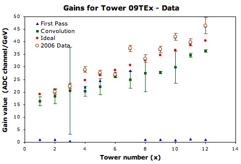
Fig. 6. Plot of the gains from 2006 data for towers in sector 9, sub-sector E.  Gain values used in Fig. 5 are also shown for comparison.

As mentioned above, the 2006 gains can be seen to be greater than the ideal gains for most of the towers in this sector and sub-sector and some of these values are significantly different from the ideal gains. 

Questions:

Does the difference observed in this sub-sector apply to others?  Is this subsector an anomaly? 

Why are the 2006 gains different from the ideal gains?

How then does this apply to the 2009 data?