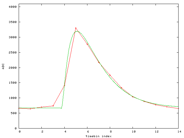
Just a simple investigation of APV pulse fits using more timebins, with an external test pulser as the signal source (negative voltage step to 0.5 pF capacitor connected to channel 12 of APV 1 on an FGT FEE board). The noise here is of course less than in case of FGT, and probably the pulse shape is significantly different as well. So, this is just for illustration.

Working in gnuplot, I made a joint fit to 15 pulses, each with independent t0 but a universal shape, baseline, and (since it is a constant-amplitude test pulse) a universal amplitude. [In real FGT pulses we can probably expect universal shape and perhaps to a reasonable approximation universal baseline too.]

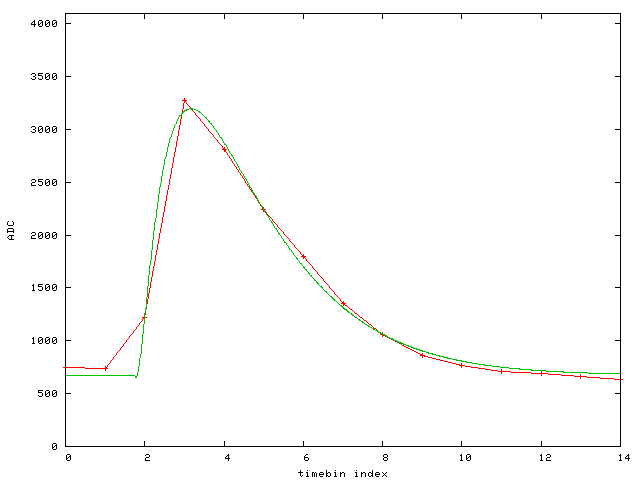
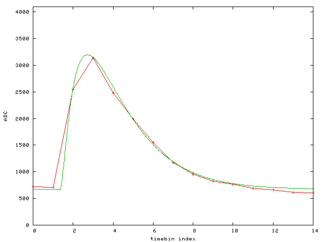
Event 1:

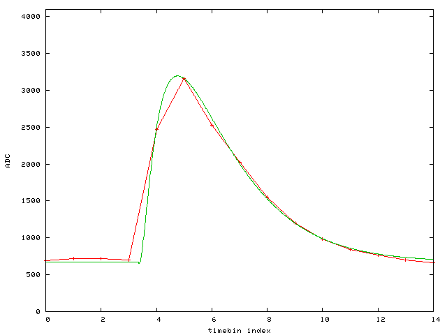
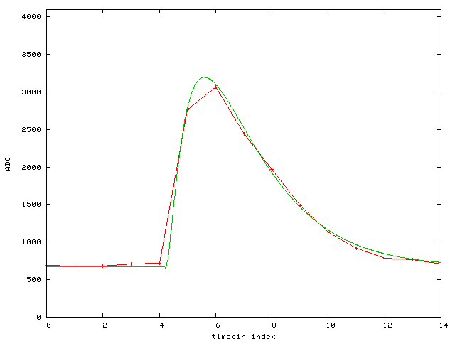
Event 2:

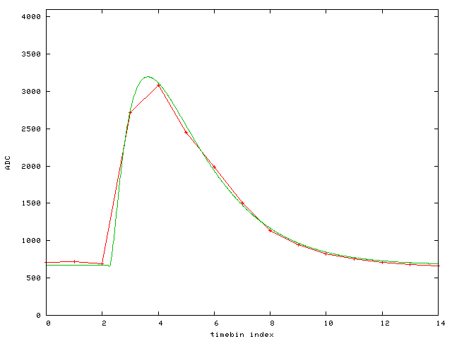
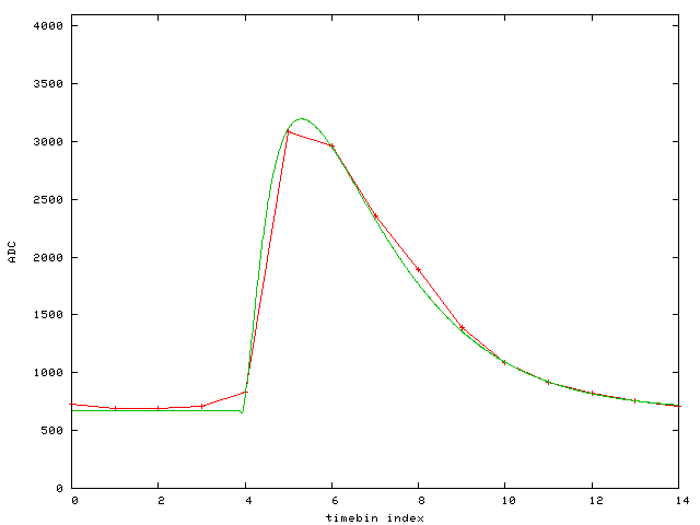
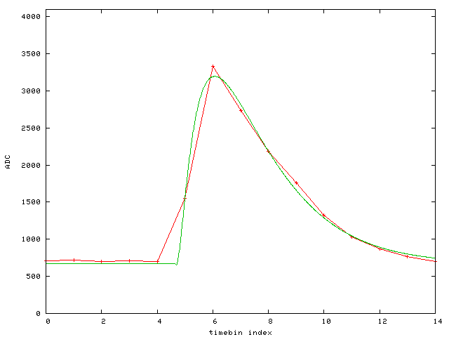
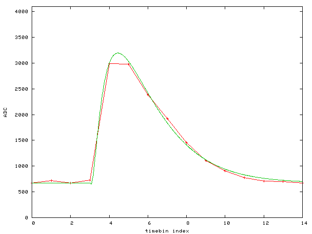
Event 3:

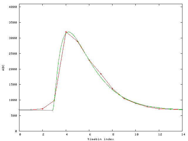
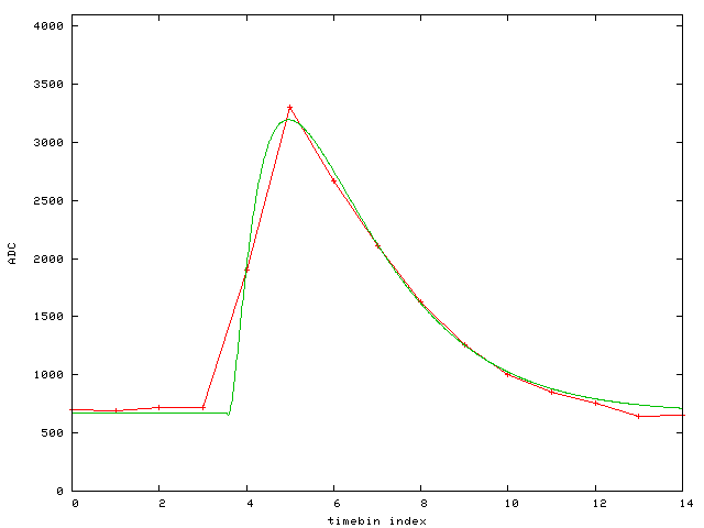
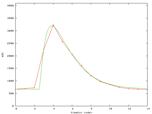
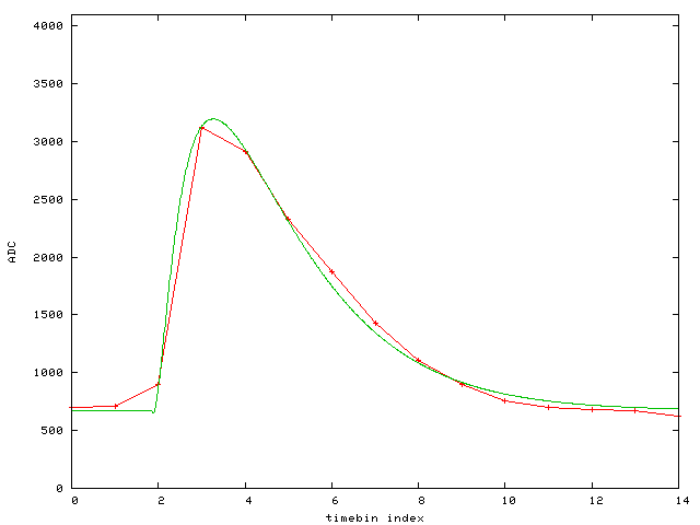
Event 4:

Event 5:

Event 6:

Event 7:

Event 8:

Event 9:

Event 10:

Event 11:

Event 12:

Event 13:

Event 14:

Event 15:

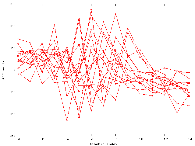
Residuals of all 15 plotted together:

The fit function is
        f(x,n)=1000*c+1000*b*(x>a(n) ? g(x-a(n)) : 0)
        g(x)=x**p*(exp(-x/tau)-m*exp(-x/tau2))

a(0) is a0 below, etc.

Fit report:
degrees of freedom (ndf) : 204
rms of residuals      (stdfit) = sqrt(WSSR/ndf)      : 47.245
variance of residuals (reduced chisquare) = WSSR/ndf : 2232.09

Final set of parameters            Asymptotic Standard Error
=======================            ==========================

a0              = 3.34421          +/- 0.5169       (15.46%)
a1              = 2.21482          +/- 0.5203       (23.49%)
a2              = 5.06759          +/- 0.5193       (10.25%)
a3              = 3.88133          +/- 0.5411       (13.94%)
a4              = 2.81781          +/- 0.5102       (18.11%)
a5              = 1.74671          +/- 0.5021       (28.75%)
a6              = 4.65391          +/- 0.5028       (10.8%)
a7              = 3.54863          +/- 0.5078       (14.31%)
a8              = 2.42739          +/- 0.5141       (21.18%)
a9              = 1.30413          +/- 0.519        (39.79%)
a10             = 4.18651          +/- 0.5197       (12.41%)
a11             = 3.03046          +/- 0.5198       (17.15%)
a12             = 1.8496           +/- 0.5195       (28.09%)
a13             = 4.77991          +/- 0.5048       (10.56%)
a14             = 3.69028          +/- 0.5019       (13.6%)
b               = 4.80118          +/- 0.1668       (3.475%)
tau             = 1.54907          +/- 0.08002      (5.165%)
p               = 0.832698         +/- 0.2247       (26.99%)
m               = 1.20295          +/- 2.375        (197.4%)
tau2            = 0.281392         +/- 0.09303      (33.06%)
c               = 0.672273         +/- 0.005485     (0.8159%)

This was just an exercise to see if a universal shape can be assumed. It seems to work ok.

Trying an individual fit with all parameters free works only for a simpler shape function, in particular x**p*exp(-x/tau), but the parameters p and tau vary over a wide range (0.6 - 1.1 for p, 1.48 - 1.76 for tau). I think it is a less correct method.

But, gnuplot is much too cumbersome to do anything further with this, so I stop this exercise. I hope it is useful as a reference for more real work with pulse shapes in FGT and IST.

Please note the shape function I used here is just an ad hoc choice, only mildly motivated by hardware considerations. There may be better forms to use for fitting.