Run6 FPD Invariant Mass Simulation and Data Comparision

With noise and digitazation effect in place, it is interesting to see how close the simulation is to the data, especially in regard to reconstruction. Here we look at the pi0 invariant mass spectrum, which is the basis for all types of FPD calibration. The categorization of events based on the topology of clusters improves the comparison, even in the absence of realistic xF-pT distribution in the simluation.

First we compare the mass spectra summed over the entire east south detector, with the usual fiducial volume cut and reconstructed di photon energy > 40GeV.

Fig. 1

The difference in mean can be fixed easily by an overall gain factor. More importantly, the simulation does a pretty good job in reproducing the sigma of the mass peak. Granted it is still about 10% smaller (peak is ~2% sharper) than the data, but the simulation only has pi0s and no other particles, with perfect calibration. (More on calibration later) The data also includes BBC vertex information, but the addition of vertex actually makes little difference in the width of the peak.

This suggests that most of the width that we see comes from reconstruction. As before, we look at the reconstructed over generated distributions for the three variables that make up the invariant mass.

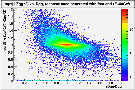
Fig2. Reconstructed over Generated, for Energy, Zgg-term, and Separaion

Clearly, most of the width is coming from the inaccuracy in reconstructing Zgg and Dgg. In fact, if the two were un-correlated, the width of the pi0 peak would be greater than what we see. But turns out they are mildly correlated.

NOTE: The Zgg term has a sharp peak at 0, which corresponds to the reconstructed energy sharing=1. This happens because of the following reason. There is a minimum energy of 2GeV for a "real" cluster. (only "real" clusters produce photons) This sets the minimum energy limit of 2GeV for a photon IF the cluster produces only one photon. But there is no such limit if the cluster produces two photons, and reconstruction sometimes conjures up essentially a zero energy photon to go with a (presumably) real photon. In fact, this was the last of the four modes of single photon splitting that were discussed in this page. 

Fig. 3

Correlation is mostly off peak, and probably related to the fact that at small Dgg-small Zgg limit, Dgg is known to be inaccurate, while at large Dgg-large Zgg limit, Zgg likely becomes inaccurate due to the limitations in measuring soft photon energy. But beyond that, it is at this point not clear to us why overestimation of separation, which usually occurs in short distances, also causes Zgg to be overestimated. (more asymmetric than it really is)

Next we look at the possiblility that the non-uniformity in cell by cell gain calibration can explain the ~2% extra sharpness of the simulation. After all, the calibration is determined up to 2% in summed energy, and some cell by cell variation is to be expected.

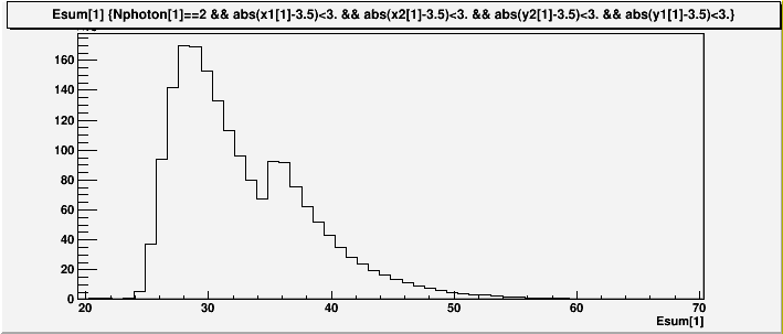
In run6, the FPD was run with summed energy trigger set nominally at 35GeV. There was also a N&S coincidence trigger set at 20GeV, which had very low rate.

Fig 4. Energy distribution for East South FPD (part of the transverse data set)

We see that the on-line calibration was in good shape for run6. For the off-line calibration, first we look at the photon position distribution for the East South, with the requirement that summed energy be greater than 40GeV, which should put us well above the trigger threshold.

Fig. 5

There are some non-uniformity, most notably at row1 column 2, but considering the very rapidly falling cross section, overall the uniformity of the distribution looks very good.

In order to quantify the uniformity of the cell by cell gain calibration for data-simulation comparison, the following scheme was tried.

Instead of looking at the invariant mass distribution by cell, we can look at it by pairs. By fixing one of the photons to be in a particular cell and varying the position of the other, in principal we get 48 mass distributions for each cell. To the extent that the calibration is uniform, these distributions should show pi0 mass peaks with similar mean value and width. 

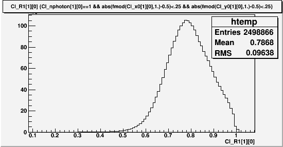
We require that each photon come from its own cluster, and the position of the cluster be in the central 0.5x0.5 square (in units of cell size) in a given cell. This requirement ensures that most of the energy of each photon comes from the cell in which the photon was reconstructed, as the highest tower on average gets ~78% of the total cluster energy. This in turn ensures that whatever variation we see in mean and sigma can be largely attributed to the particular cell in the pair, if indeed such variations are due the non-uniformity in cell by cell calibration.

Fig. 6 Fraction of the energy in the highest tower for the "central" clusters

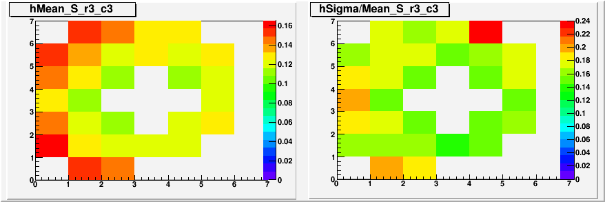
With this condition, here is an example of what the mean value and sigma of the pi0 mass peak look like for the South row3 column3 when paired with all other cells that have sufficient statistics to allow the fitting. There is no software trigger, so the samples are dominated by low energy events. (We expect low mass here as there is no energy dependent correction)

Fig. 7 Mean and Sigma/Mean of pi0 peak distribution for various pairs, with the fixed cell at r3 c3. Gaussian fit was done from 0.07GeV~0.2GeV.

The absence of directly neighboring cells is likely due to the requirement that each photon have its own cluster. There is also a general trend where pairing with far away cells (distance>3 cell) produces abnormally higher mass. It can be understood as a trigger bias, as the rapidly falling cross section means that most of these events have similar energy, and separation correlates well with mass after that. Therefore we confine the comparison to the 12 cells that are 2~sqrt(5) cell width away from the central cell, which roughly corresponds to symmetric decays for ~25GeV-ish pi0s.

The RMS of the means is to some extent a measure of gain uniformity for these 12 cells. We can also look at the distribution of gaussian sigmas, which is a measure of mass resolution for specific pairs. We can compare these quantities from data against those from simulation with perfect calibration to see if the differences can be understood as the result of gain non-uniformity.

Fig. 8 Distribution of RMS of gaussian centroids, normalized to pi0 mass. Left hand side is the data, and right hand side is the simulation.

The simulation is very much limited in statistics compared to the low energy data. Consequently the quality of fit was much lower with the simulation, and that is clearly affecting the results. Nonetheless, we can still see that ~3.5% of pairing dependent spread in centroids seen in data is likely not due to the gain non-uniformity, as the simulation with perfectly uniform calibration doesn't seem to do any better. The relatively small spread of centroids (little contribution to the peak width) is also consistent with the earlier finding that most of the width in the mass spectrum can be understood in terms of how reconstruction works.

Next we look at the mean of the gaussian sigmas, which is a measure of mass resolution. 

Fig. 9 Distribution of mean of gaussian sigmas divided by the mean. Left hand side is the data, and right hand side is the simulation.

Here we see that the width of mass peaks on average is about 2.5% sharper for the simulation, while the data has average width of ~15%. This is consistent with what we expect from our analysis of the overall mass resolution.

In order to verify the effect of gain non-uniformity, I added (3/sqrt(2))% random variation in energy to the simulation and looked at the same quantities. The result was that it actully changes things very little. There was no significant increase in the spread, both for the centroid and the sigma, and these numbers actually improved slightly.

Apparently, a few percent random variation in gain corrections have little effect in the di-photon mass distributions, and cannot explain the 2% extra sharpness observed in the simulation. However, there are likely a lot of room for improvement on how this pair-wise fitting is done, as these numbers can be changed quite easily by how many cells we include in the fit. What remains true, though, is that in most cases, the simulation tracks the data quite well.