Final Stretch

The calibration is more or less complete. I have found a couple of issues, which I am working on now, but they are unlikely to change the cross-section result in any meaningful way. 

As discussed many times before, the energy smearing turned out to be much worse than we expected. This introduces an ambiguity in calibration. The point of calibration is of course to make the mean of the reconstructed to thrown energy ratio to be close to one. I could either do it in apparent energy bins, or I could do it in thrown energy bins. They are not the same, due to the bin migration caused by crappy energy resolution. Either case, the simulation has to match the data well, not just event by event, but also in the overall shape of the cross-section, to properly deal with the bin migration.

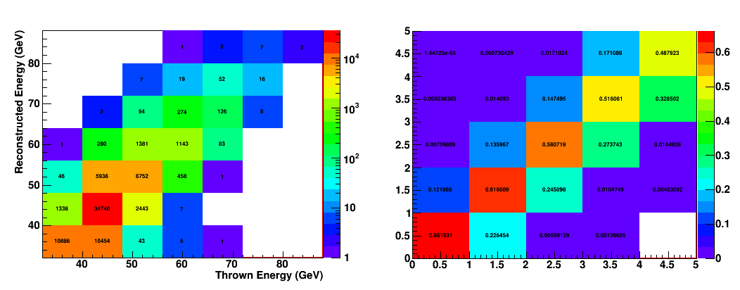
If I calibrate in apparent energy bins, then the nice thing is that the mean energy in each measured energy bin is automatically correct. The bad thing is that now the calibration is cross-section and binning dependent. This is because I have folded in the bin migration into the calibration. It also makes the smearing matrix very non-diagonal and asymmetrical, which is kind of nasty.

So I calibrated in thrown energy bins, which results in the mean energy being correct when binned in true energy. That is, it is more of an absolute calibration that works for individual photons, regardless of the cross-section. But the mean energy measurement in measured energy bins would be somewhat overestimated, due to bin migration. But this method produces a micer smearing matrix.

All of this makes more sense with a picture.

Fig. 1. Reconstructed vs. Thrown energy distribution for pi0's, and the resulting smearing matrix.

If Vrec is the vector of measured energy distribution, and Vtrue is the  vecctor of true energy distribution, and S the smearing matrix, then we have,

Vrec = S Vtrue

An obvious thing to do is then to invert S, and apply it to the Vrec from data. This actually doesn't work as well as I expected, mostly due to the fact that the matrix is really not that diagonal or symmetric, and there are errors in the matrix itself. I am left with infinite number of true energy distributions that are consistent with our limited understanding of the smearing. All of those are qualitatively similar, but not the same.

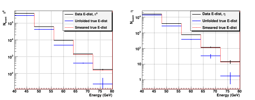
So I go the other way. I assume some form of cross-section, which is an exponential with cubic argument, so that it may fall a little faster than a regular exponential. This is actually a very loose requirement, and it pretty much amounts to asking for smoothness. I get a distribution from this function, which is my Vtrue, multiply it by S, and I get my Vrec. This is my fit function. I let the parameters of this function vary, and I fit it against the actual measured distribution in data. 

Fig. 2. Result from smearing matrix fit. 

The red lines are my "function" which is fit against the black distribution underneath. The blue distribution is my "true" energy distribution, based on the result of the fit. 

I'd like to emphasize once again that if I go with the matrix inversion, the result is not outrageously different at lower energy bins. But it's very easy to  change the very last bin significantly, for example. This says that given the smearing, and my simulation statistics, we really have very little measurement in that bin. This has to go into the systematic error.

Using this result, here are what the absolute and relative cross-section look like at this stage. I used 6.8pb-1 int. luminosity for convenience. I have not included the systematics due to the error in my mixing matrix. But I did "overestimated" my energy scale error to be safe. (I'm using 3% absolute and 2% relative calibration uncertainty)

Fig. 3. Absolute cross-section estimate.

I am still checking all my formulas and scripts. There is still a chance that I've done something wrong, and the results agree better with the previous ones. In the mean time, I'll list some of the main differences between the previous analysis and mine.

1. Cerenkov based simulation produces much worse energy resolution. Energy deposition gives you ~1% energy resolution. Cerenkov gives you ~1.5% if the glass has no attenuation, but with realistic attenuation, we get ~8%. The reason that we believe this to be a better estimate is because,

          a. Energy dependent mass shift is better simulated, and fully understood. It comes from the actual shift in gain (which doesn't exist in energy loss simulation) plus the energy bin migration due to poor resolution. (which is negligible with 1% resolution)

          b. The width of the mass peak in simulation matches the data much better with Cerenkov. 

2. Shower function is different. While the new one isn't perfect, it matches the data better, and it has incident angle dependence. The previously simulated energy dependent mass shift with energy loss based Geant was mostly coming from the energy dependent shift in separation, which has been eliminated with the new shower shape and some modification to reconstruction.

3. To account for the bin migration, now we unfold the energy distribution using the mixing matrix. This results in a distribution that falls faster. We also calibrate in a way that doesn't fold in the bin migration. The exact consequence of these differences are difficult to tell, since it all depends on how it was calibrated. 

4. All in all, I have not found a single thing that matches the data worse after I switched to Cerenkov.  I do believe Cerenkov is the way to go.

We can also look at the cross-section ratio, but this may be affected more by the remaining issue in calibration, and also the precise form of the function I use to guide the true distribution. Again, only some portion of the systematics have been included.

Fig. 4. Cross-section ratio estimate

And finally, we want to look at the asymmetry. However, the remaining issues in calibration may actually have some impact on the asymmetry result, at very high energy. The statistics we are playing with is very small, and every event counts. So this result may change in a day or two. Furthermore, I find that it's actually rather easy to mess with the significance of the result by doing fairly benign things like changing mass cuts and center cut slightly. I am investigating that as well. 

I am also starting to go through event by event comparison between old and new results. So far the only things that I've notice is that I am throwing away three photon events, even when the third photon is very very soft. 

Fig. 5. AN estimate