EPD calibration for Au+Au 2017 (and method in general)
Updated on Thu, 2017-10-12 17:20. Originally created by lisa on 2017-10-12 13:02.
Overview:
Each tile in the EPD returns an ADC value for every event. To use these in an ADC-weight-based analysis, the gains of the tiles must be matched. We can do this to an extent by adjusting the bias voltage on the SiPM during the run, but there will always need to be some offline calibration. Here, I will go through the calibration procedure. Along the way, we will see that the 93 tiles in the 2017 run behaved in a very well-understood way.
Assuming a linear relationship between (average) energy lost in the tile and ADC value (see here for the assumptions involved in this), then
dE = Gain*(ADC+offset) (Eq 1)
The ADC distributions all follow Landau expectations
We are not really interested in the energy deposited in keV, but rather want a measure of the number of particles (we assume all are MIPs, even though some low-p stuff is going to spiral in) that traverse a tile. As I have shown before, a MIP generates on average about 40-50 photelectrons. The Poisson fluctuations for this number are small relative to the width of the energy loss distribution in 1.2 cm of scintillator, given by the Landau distribution. Therefore, in what follows, I will ignore Poisson fluctuations (they can be included, but it is a pain) and ask whether the ADC distribution, which is linearly related to the energy loss distribution, can be described by the Landau expectation.
They can. Here are the raw ADC distributions (here, the offset was not accounted for, but that is tiny on this scale) for all 93 tiles. It is too small to read (sorry, maybe I'll update later), but the x-axis has been autoscaled. It is different for each tile. You can download the pdf of all tiles, (or else right-click on the image to "view") and zoom in if you want.
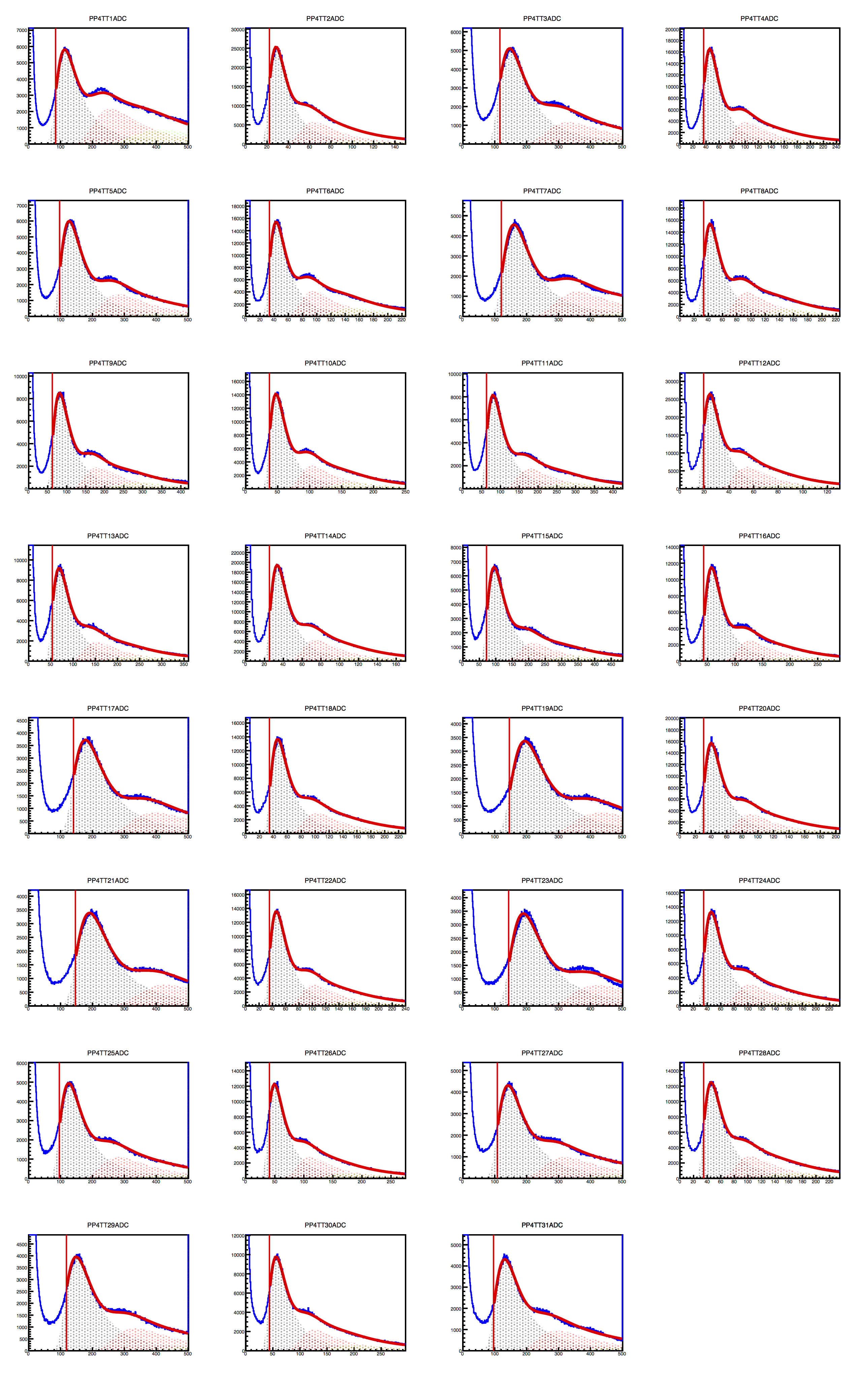
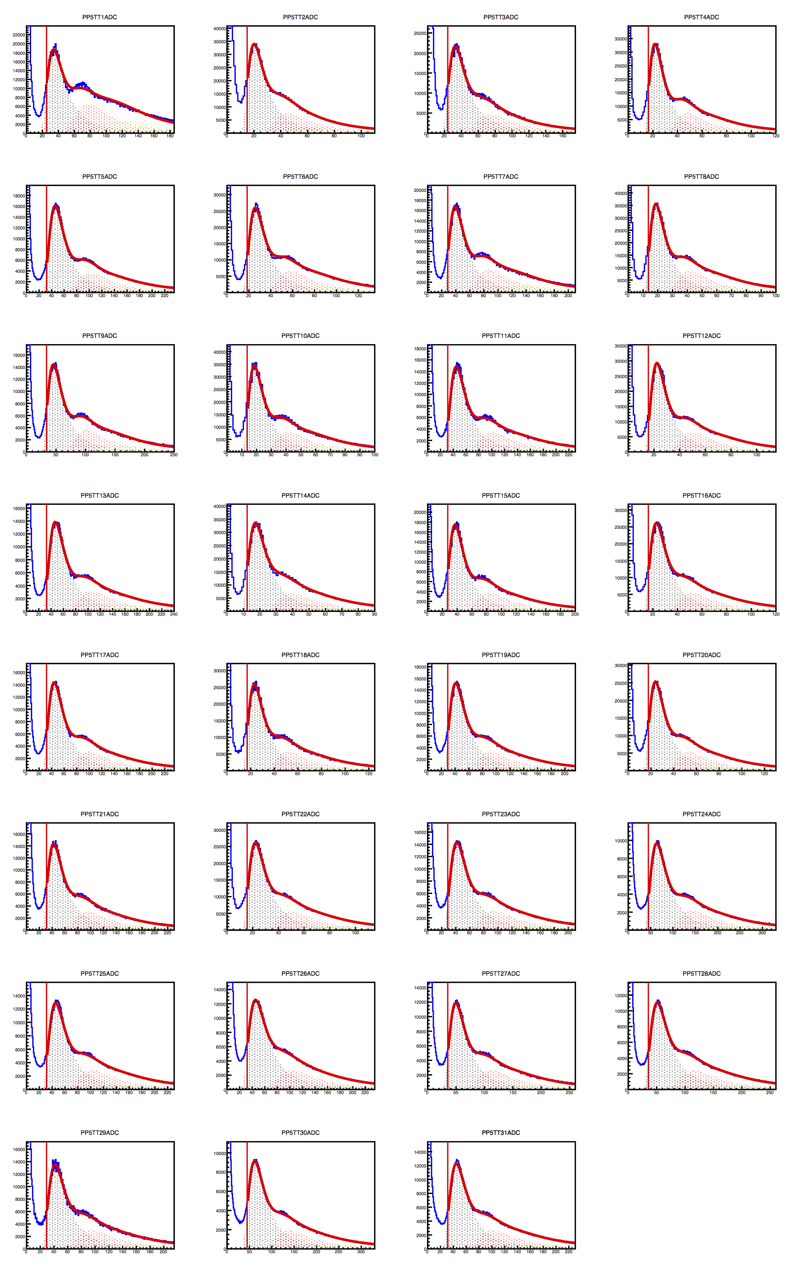
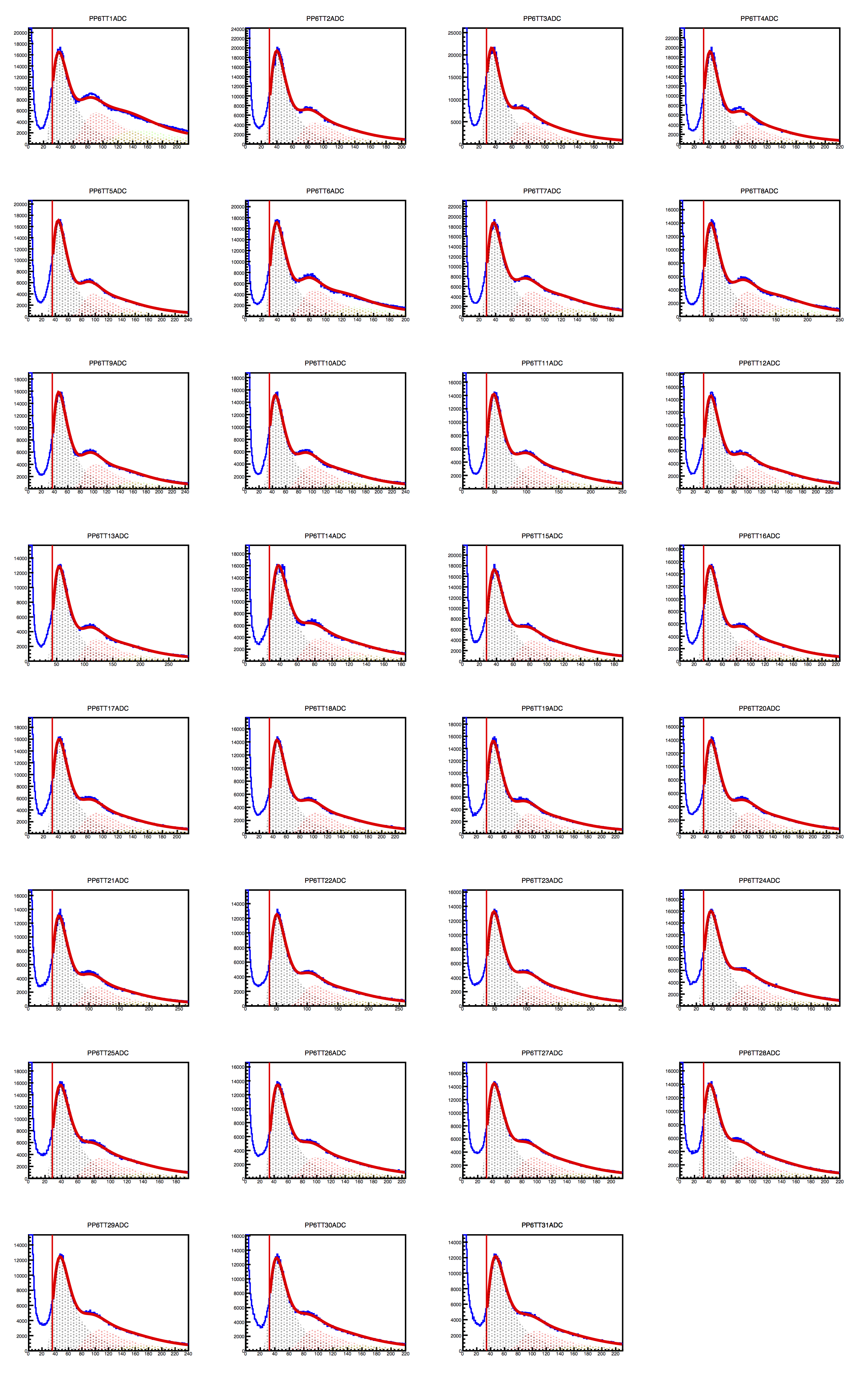
Figure 1 - raw ADC distributions for supersectors at positions 4 (left), 5 (middle) and 6 (right), from the 2017 Au53Au run. The horizontal axis is ADC value, and it is autoscaled. The peaks occur at different ADC values for the different tiles. Red solid line represents a multiple-Landau fit. Shaded regions show 1-, 2- and 3-MIP contributions. The spectrum to the left of the vertical red line is not included in the fit.
In the above, the red curve is the contribution of 1-, 2- and 3-MIP distributions. The individual contributions are shown as shaded regions. The parameters in the fit are
The fits are not perfect. As I have discussed with Les Bland, there is commonly a "low-ADC shoulder" on the single-MIP distribution. This may come from position-dependent response of the tile, or from particles passing through only part of a tile (which amounts to the same). Also, there should after all be some Poisson broadening, and this will be larger for the 1-MIP distribution than N-MIP (N>1). We may investigate this. For now, we recognize the fits to be perfect, but use them as starting points to gain-equalize.
The MPV and offset values for each tile comes from these fits and are entered into the STAR database (managed for the EPD by Prashanth) for calibration. The calibration constants are given below or can be downloaded here.
Gain equalization and going from ADC to number of MIPs
We will express the calibrated data in terms of "nMIP",
where ADC is the value that comes directly from the STAR DAQ, offset has been discussed above, and "MIP" is actually the MPV for the 1-MIP Landau distribution. Hence, nMIP is the energy loss in units of the MPV for a single ionizing particle.
Here are the nMIP distributions, for the 93 tiles. (Again in this plot, the small offset has been neglected.) These appear identical to the ones above, but they are not. The x-axis is now the same for all tiles (nMIP) and there is no autoscaling. You can download the pdf here and blow it up if you like.
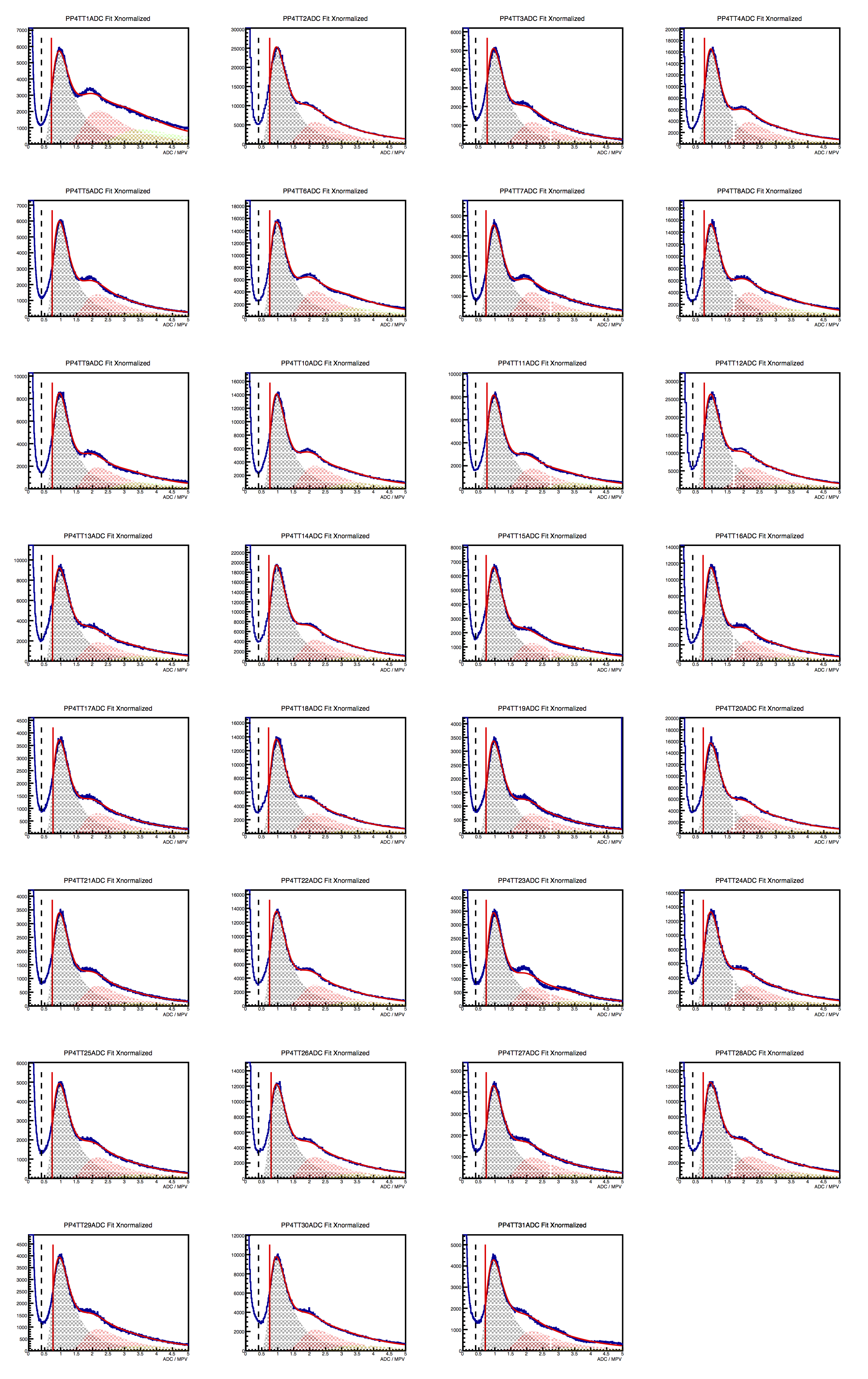
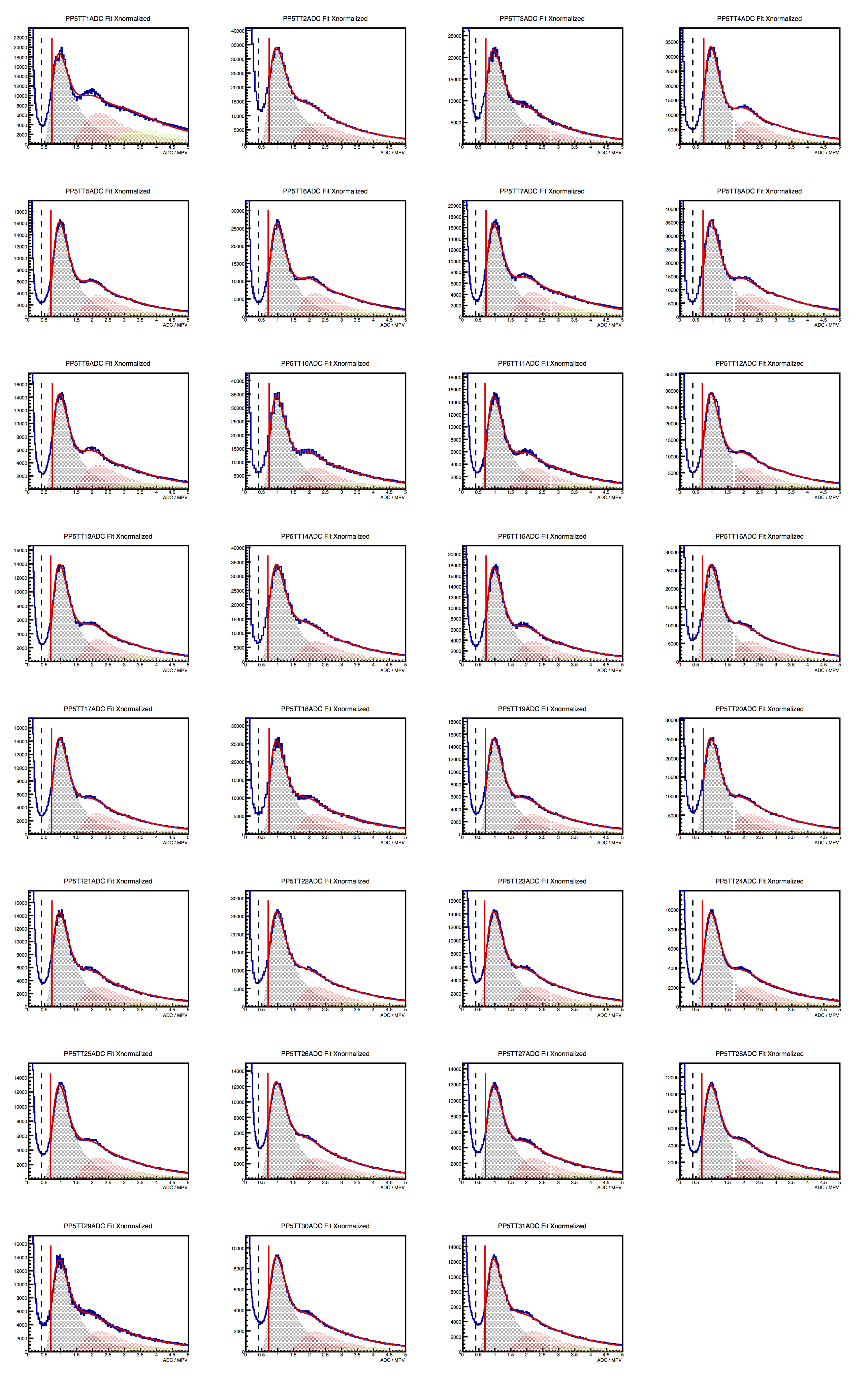
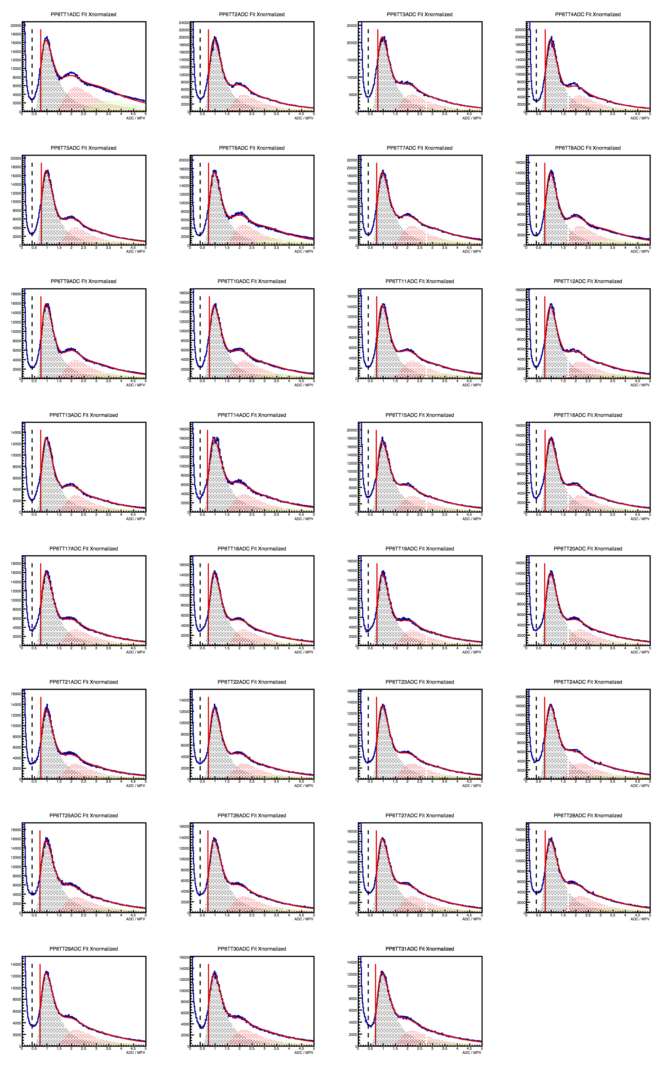
Figure 2 - ADC/MPV distributions for supersectors at positions 4 (left), 5 (middle) and 6 (right), from the 2017 Au53Au run. The horizontal axis is nMIP, and it is not autoscaled. Red solid line represents a multiple-Landau fit. Shaded regions show 1-, 2- and 3-MIP contributions. The spectrum to the left of the vertical red line is not included in the fit. Vertical dashed line is a suggested threshold value, to cut out dark current. It is shown just to emphasize that one single threshold value could apply to all 93 tiles, in this space.
It really really makes sense.
So far, so good. 93 out of 93 tiles make good sense, and we can gain-equalize. Keeping in mind the tile layout of the EPD (below), we can identify 16 "rings." Ring 1 is composed of all the TT01, and Ring 16 is composed of all the TT30 and TT31. In 2017, each ring had 6 tiles except for ring 1 which only had 3.
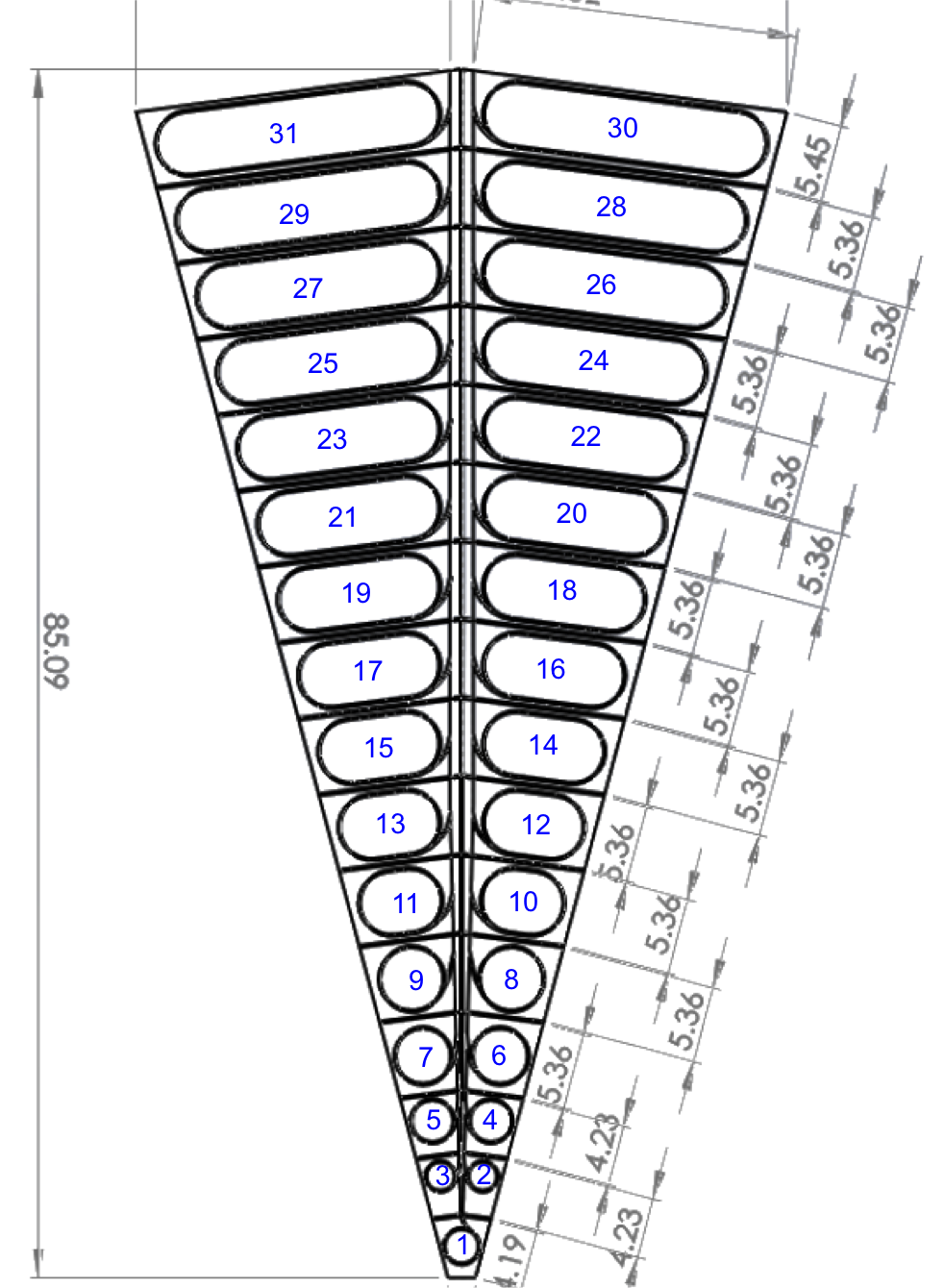
Figure 3 - A reminder of the tile layout. Tiles 2 and 3 cover same eta range, so can be considered in the same "Ring." Likewise for tiles 20 and 21. There are 16 rings.
Naturally, one expects the "same" nMIP spectrum from all tiles in a given ring. As seen here, this is clearly not true for the ADC distributions.....

Figure 4 - The 93 tiles in the 2017 run are shown grouped in Rings of common eta range. Clearly, the ADC distributions are different in both vertical and horizontal directions (pdf file here)
... but the nMIP distributions do coincide very well!
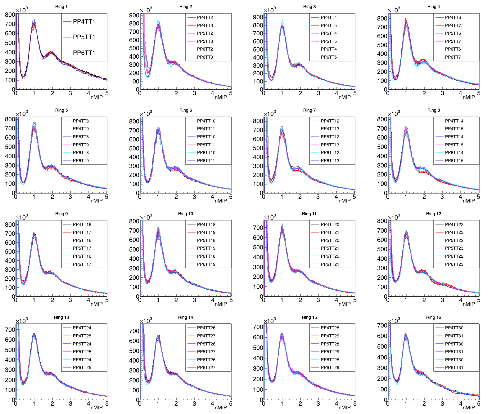
Figure 5 - nMIP distributions for all 93 tiles in the 2017 run, grouped into 16 Rings of common eta range. (pdf file here)
Now, consider. The only thing that has changed Figure 4 into Figure 5 was applying the linear relationship from equation 2 above. (And since offset is very small, it is basically only a scaling.) So, the only "trivial" thing about the agreement above is that the 1-MIP peak must be the same for all plots. What is not trivial:
One can also look at the heights of the 1-, 2- and 3-MIP peaks as a function of eta, and things make systematic sense.
(It is noted that the agreement of the spectra is impressive but not perfect. In particular, some of the odd-numbered tiles from PP04 look strange, especially PP04TT23, but also TT15 and TT31. These tiles were read out by QT32Cs and they are separated by eight channels, and this looks like an electronics issue, so I will be looking more into that.)
Summary:
Unit offset in Run 2017 data
Akio wrote up the problem here.
In an email exchange with me, Rosi and Gerard, he made it explicit:
I think it will be very small effect for EPD and can ignore.
Essentially ADC recorded is 1 count too small, and you need to add 1 to get it correct.
(I assume you are not using bitgain shift). For a single cell, it has small impact.
For FMS cluster/jet which adds ADC for 20 cells, its off by 20 count
which causes none-linearliry (and we use bitgain shift to make
it worse).
(Akio's assumption that we do not use bitgain shift is correct.)
Correction that should be implemented
The calibration above normalizes the gains, tile-to-tile. However, there is another issue which may be small, or not. It should be investigated.
In particular, a larger ADC value is assigned a larger nMIP value in our scheme. However, consider one tile, with one particle passing through it. If the particle passes through with normal incidence, it traverses 1.2 cm of scintillator (the thickness of our detector). However, if it crosses at an angle, then it traverses more scintillator and will leave more energy, and the ADC spectrum will be shifted (and broadened) relative to the normal-incidence case. Larger incidence angle will occur for collisions that occur nearer to the detector (keep in mind that the vertex position is not fixed).
What needs to be done is to look at the ADC distribution for events that occur close to the detector and those that occur far away, to gauge the size of this effect. We could probably work up a Vz-dependent correction if we want. I have not done this.
Fitting with multiple convoluted Landaus:
In root v6, here is the function you can use, to fit an ADC distribution
Calibration constants for the Run 2017 Au+Au run
Overview:
Each tile in the EPD returns an ADC value for every event. To use these in an ADC-weight-based analysis, the gains of the tiles must be matched. We can do this to an extent by adjusting the bias voltage on the SiPM during the run, but there will always need to be some offline calibration. Here, I will go through the calibration procedure. Along the way, we will see that the 93 tiles in the 2017 run behaved in a very well-understood way.
Assuming a linear relationship between (average) energy lost in the tile and ADC value (see here for the assumptions involved in this), then
dE = Gain*(ADC+offset) (Eq 1)
where the calibration constants are shown in blue. Since we pedestal-subtract, one expects offset to be (close to) zero. However, due to a technical issue (see here for details), there was an offset of 1 count for all of our ADCs. I.e. when we see "ADC=1" in the data, that means two counts above pedestal. This is a small effect, but some of our MIP peaks are around 40 or so, so it can matter a bit.
A big thanks to Xinyue Ju for running over the data and extracting these calibration constants.
The ADC distributions all follow Landau expectations
We are not really interested in the energy deposited in keV, but rather want a measure of the number of particles (we assume all are MIPs, even though some low-p stuff is going to spiral in) that traverse a tile. As I have shown before, a MIP generates on average about 40-50 photelectrons. The Poisson fluctuations for this number are small relative to the width of the energy loss distribution in 1.2 cm of scintillator, given by the Landau distribution. Therefore, in what follows, I will ignore Poisson fluctuations (they can be included, but it is a pain) and ask whether the ADC distribution, which is linearly related to the energy loss distribution, can be described by the Landau expectation.
They can. Here are the raw ADC distributions (here, the offset was not accounted for, but that is tiny on this scale) for all 93 tiles. It is too small to read (sorry, maybe I'll update later), but the x-axis has been autoscaled. It is different for each tile. You can download the pdf of all tiles, (or else right-click on the image to "view") and zoom in if you want.
Figure 1 - raw ADC distributions for supersectors at positions 4 (left), 5 (middle) and 6 (right), from the 2017 Au53Au run. The horizontal axis is ADC value, and it is autoscaled. The peaks occur at different ADC values for the different tiles. Red solid line represents a multiple-Landau fit. Shaded regions show 1-, 2- and 3-MIP contributions. The spectrum to the left of the vertical red line is not included in the fit.
In the above, the red curve is the contribution of 1-, 2- and 3-MIP distributions. The individual contributions are shown as shaded regions. The parameters in the fit are
- the ADC value for the MPV (most probable value) of the Landau distribution
- the WID/MPV of the Landau distribution (expected to be about 0.14-0.16, and it always is)
- the number of 1-, 2- and 3-MIP events
The fits are not perfect. As I have discussed with Les Bland, there is commonly a "low-ADC shoulder" on the single-MIP distribution. This may come from position-dependent response of the tile, or from particles passing through only part of a tile (which amounts to the same). Also, there should after all be some Poisson broadening, and this will be larger for the 1-MIP distribution than N-MIP (N>1). We may investigate this. For now, we recognize the fits to be perfect, but use them as starting points to gain-equalize.
The MPV and offset values for each tile comes from these fits and are entered into the STAR database (managed for the EPD by Prashanth) for calibration. The calibration constants are given below or can be downloaded here.
Gain equalization and going from ADC to number of MIPs
We will express the calibrated data in terms of "nMIP",
nMIP = (ADC + offset)/MIP (Eq 2)
where ADC is the value that comes directly from the STAR DAQ, offset has been discussed above, and "MIP" is actually the MPV for the 1-MIP Landau distribution. Hence, nMIP is the energy loss in units of the MPV for a single ionizing particle.
Here are the nMIP distributions, for the 93 tiles. (Again in this plot, the small offset has been neglected.) These appear identical to the ones above, but they are not. The x-axis is now the same for all tiles (nMIP) and there is no autoscaling. You can download the pdf here and blow it up if you like.
Figure 2 - ADC/MPV distributions for supersectors at positions 4 (left), 5 (middle) and 6 (right), from the 2017 Au53Au run. The horizontal axis is nMIP, and it is not autoscaled. Red solid line represents a multiple-Landau fit. Shaded regions show 1-, 2- and 3-MIP contributions. The spectrum to the left of the vertical red line is not included in the fit. Vertical dashed line is a suggested threshold value, to cut out dark current. It is shown just to emphasize that one single threshold value could apply to all 93 tiles, in this space.
It really really makes sense.
So far, so good. 93 out of 93 tiles make good sense, and we can gain-equalize. Keeping in mind the tile layout of the EPD (below), we can identify 16 "rings." Ring 1 is composed of all the TT01, and Ring 16 is composed of all the TT30 and TT31. In 2017, each ring had 6 tiles except for ring 1 which only had 3.
Figure 3 - A reminder of the tile layout. Tiles 2 and 3 cover same eta range, so can be considered in the same "Ring." Likewise for tiles 20 and 21. There are 16 rings.
Naturally, one expects the "same" nMIP spectrum from all tiles in a given ring. As seen here, this is clearly not true for the ADC distributions.....
Figure 4 - The 93 tiles in the 2017 run are shown grouped in Rings of common eta range. Clearly, the ADC distributions are different in both vertical and horizontal directions (pdf file here)
... but the nMIP distributions do coincide very well!
Figure 5 - nMIP distributions for all 93 tiles in the 2017 run, grouped into 16 Rings of common eta range. (pdf file here)
Now, consider. The only thing that has changed Figure 4 into Figure 5 was applying the linear relationship from equation 2 above. (And since offset is very small, it is basically only a scaling.) So, the only "trivial" thing about the agreement above is that the 1-MIP peak must be the same for all plots. What is not trivial:
- not only the position of the 1-MIP peak lines up, but the entire shape of the spectrum. Widths of peaks, inflections, etc.
- also, there is no vertical "normalization" in these plots. The heights of the peaks (not only the relative heights, but the heights) are meaningful, not only within a ring, but even going from ring to ring. Keep in mind that a Jacobian (1/MPV) must be applied when going from figure 4 to figure 5.
One can also look at the heights of the 1-, 2- and 3-MIP peaks as a function of eta, and things make systematic sense.
(It is noted that the agreement of the spectra is impressive but not perfect. In particular, some of the odd-numbered tiles from PP04 look strange, especially PP04TT23, but also TT15 and TT31. These tiles were read out by QT32Cs and they are separated by eight channels, and this looks like an electronics issue, so I will be looking more into that.)
Summary:
- All 93 tiles used in the Au+Au run of 2017 worked well and their behavior is understood. Certain small discrepancies remain.
- A first calibration has been produced and is entered into the database.
- muDSTs and picoDSTs read with StEpt will provide the user with calibrated nMIP data for each tile. Analysis will be easy. No need to deal with ADCs in most cases.
- Nphotons produced proportional to dE - yes
- Nphotons transported to SiPM proportional to Nphotons produced - assumed yes (hard to think otherwise)
- Nelectrons generated proportional to Nphotons impinging on SiPM - yes, as long as Nphoton << Npixels illumimnated. For us that is ~50 << 1662
- Linear gain of SiPM - very good, according to Hamamatsu
- Linear gain of FEE - very good, according to Gerard
- Linear gain of QT board - very good, according to Steve
Unit offset in Run 2017 data
Akio wrote up the problem here.
In an email exchange with me, Rosi and Gerard, he made it explicit:
I think it will be very small effect for EPD and can ignore.
Essentially ADC recorded is 1 count too small, and you need to add 1 to get it correct.
(I assume you are not using bitgain shift). For a single cell, it has small impact.
For FMS cluster/jet which adds ADC for 20 cells, its off by 20 count
which causes none-linearliry (and we use bitgain shift to make
it worse).
(Akio's assumption that we do not use bitgain shift is correct.)
Correction that should be implemented
The calibration above normalizes the gains, tile-to-tile. However, there is another issue which may be small, or not. It should be investigated.
In particular, a larger ADC value is assigned a larger nMIP value in our scheme. However, consider one tile, with one particle passing through it. If the particle passes through with normal incidence, it traverses 1.2 cm of scintillator (the thickness of our detector). However, if it crosses at an angle, then it traverses more scintillator and will leave more energy, and the ADC spectrum will be shifted (and broadened) relative to the normal-incidence case. Larger incidence angle will occur for collisions that occur nearer to the detector (keep in mind that the vertex position is not fixed).
What needs to be done is to look at the ADC distribution for events that occur close to the detector and those that occur far away, to gauge the size of this effect. We could probably work up a Vz-dependent correction if we want. I have not done this.
Fitting with multiple convoluted Landaus:
In root v6, here is the function you can use, to fit an ADC distribution
TF1* func = new TF1("MultiMipFit",myfunc,xlo,xhi,nMipsMax+2);
MipPeak[0] = new TF1("1MIP","TMath::Landau(x,[0],[1],1)",xlo,xhi);
for (Int_t nMIP=2; nMIP<=nMipsMax; nMIP++){
TF1Convolution* c = new TF1Convolution(MipPeak[nMIP-2],MipPeak[0],xlo,xhi,true);
MipPeak[nMIP-1] = new TF1(Form("%dMIPs",nMIP),c,xlo,xhi,2*nMIP);
}
for (Int_t nmip=0; nmip<nMipsMax; nmip++){
func->SetParName(nmip,Form("%dMIPweight",nmip+1));
func->SetParLimits(nmip,0.0,1e8); // MIP weight
}
func->SetParName(nMipsMax,"MPV");
func->SetParName(nMipsMax+1,"WIDbyMPV");
func->SetParameter(nMipsMax+1,0.13);
func->SetParLimits(nMipsMax+1,0.11,0.22); // WIDbyMPV ~ 0.16
Calibration constants for the Run 2017 Au+Au run
PP SS MIP Offset
4 1 119.345 1
4 2 30.5225 1
4 3 153.404 1
4 4 48.1599 1
4 5 132.55 1
4 6 45.2512 1
4 7 167.186 1
4 8 44.8508 1
4 9 84.8077 1
4 10 49.8178 1
4 11 84.0953 1
4 12 26.1976 1
4 13 72.1517 1
4 14 35.6139 1
4 15 99.0508 1
4 16 60.0672 1
4 17 184.907 1
4 18 48.5573 1
4 19 201.775 1
4 20 42.4804 1
4 21 198.599 1
4 22 48.5286 1
4 23 197.056 1
4 24 48.5641 1
4 25 131.636 1
4 26 52.2454 1
4 27 148.751 1
4 28 48.7242 1
4 29 156.179 1
4 30 59.2571 1
4 31 137.891 1
5 1 36.429 1
5 2 22.2165 1
5 3 35.2395 1
5 4 23.5009 1
5 5 48.3144 1
5 6 27.9255 1
5 7 41.6368 1
5 8 20.3628 1
5 9 48.3619 1
5 10 20.1177 1
5 11 47.3776 1
5 12 24.1149 1
5 13 49.6286 1
5 14 19.1904 1
5 15 39.5841 1
5 16 24.9074 1
5 17 46.9243 1
5 18 25.0556 1
5 19 43.6414 1
5 20 25.7726 1
5 21 45.2 1
5 22 23.9779 1
5 23 44.197 1
5 24 67.1734 1
5 25 48.3771 1
5 26 48.5835 1
5 27 52.6688 1
5 28 54.383 1
5 29 44.6191 1
5 30 65.3251 1
5 31 47.6924 1
6 1 43.3127 1
6 2 42.0974 1
6 3 37.5177 1
6 4 43.675 1
6 5 46.6546 1
6 6 40.8373 1
6 7 39.7532 1
6 8 50.686 1
6 9 48.6937 1
6 10 46.7565 1
6 11 50.7233 1
6 12 47.7025 1
6 13 57.1614 1
6 14 40.2392 1
6 15 39.7072 1
6 16 45.0289 1
6 17 43.3678 1
6 18 48.5292 1
6 19 46.1112 1
6 20 48.8551 1
6 21 52.9183 1
6 22 53.4168 1
6 23 51.1888 1
6 24 40.1143 1
6 25 41.0821 1
6 26 47.5768 1
6 27 44.6763 1
6 28 43.866 1
6 29 50.0068 1
6 30 45.1329 1
6 31 49.9069 1
»
- lisa's blog
- Login or register to post comments