First heat map of SS06
Updated on Sun, 2017-08-27 23:16. Originally created by lisa on 2017-08-27 20:31.
We are using a 200 microCi Sr90 source, mounted on an x-y table, to measure the response of the detector as a function of position. Our 1.2-cm-thick detector (with wrapping) is too thick for any appreciable flux of particles passing through to the other side. Therefore, we are not looking at triggered particles, but rather untriggered dark current, as reported by the FEEs when queried by the TUFF box.
When the source is held close to the supersector, we have seen about a 200 nA rise in dark current in the close tile. I've described this here. In the current test, in order to hold the SS relatively flat, it is held by a piece of foamboard atop stretched nylon. In this configuration, the increase in dark current is only on order 100 nA.
We are biasing the SiPMs at 56 V (about what we used in the 2017 run). They have been irradiated, so have dark current of about 1.1 uA.
Procedure:
A full set of plots may be found here
This scanning set-up is NOT trivial, and I feel the need to identify work done by many individuals over months
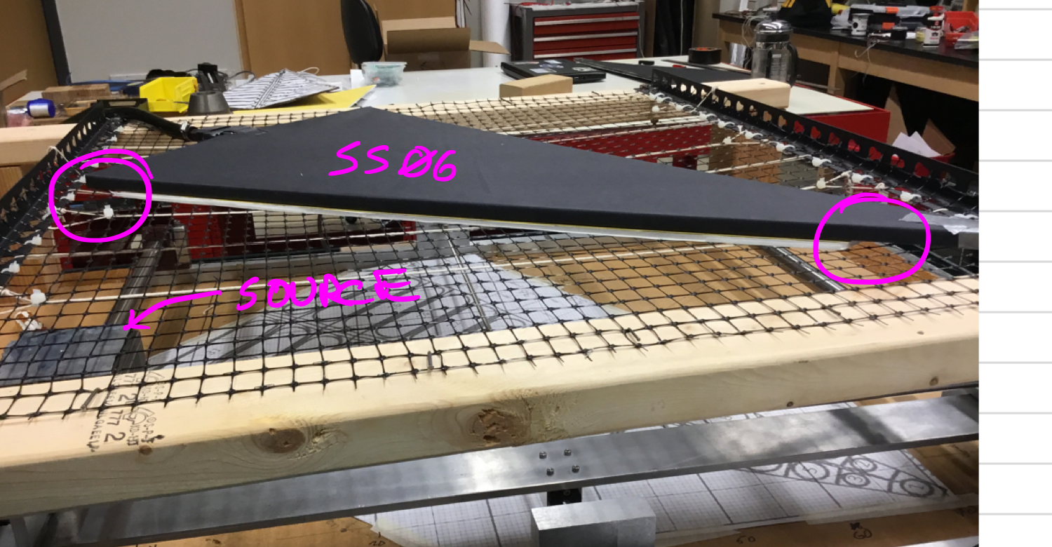
Figure 1 - Supersector 06 sits on a foam board atop a stretched nylon netting. The Sr90 source is mounted on an xy table; it is at lower left in the photo. The source is about 1 cm below the supersector when positioned underneath.
Here, I report the first scan of SS06, stepping by 2 cm in x and 4 cm in y. I used 96 positions, focusing on the large-number tiles. The approximate location of the positions sampled is shown below.
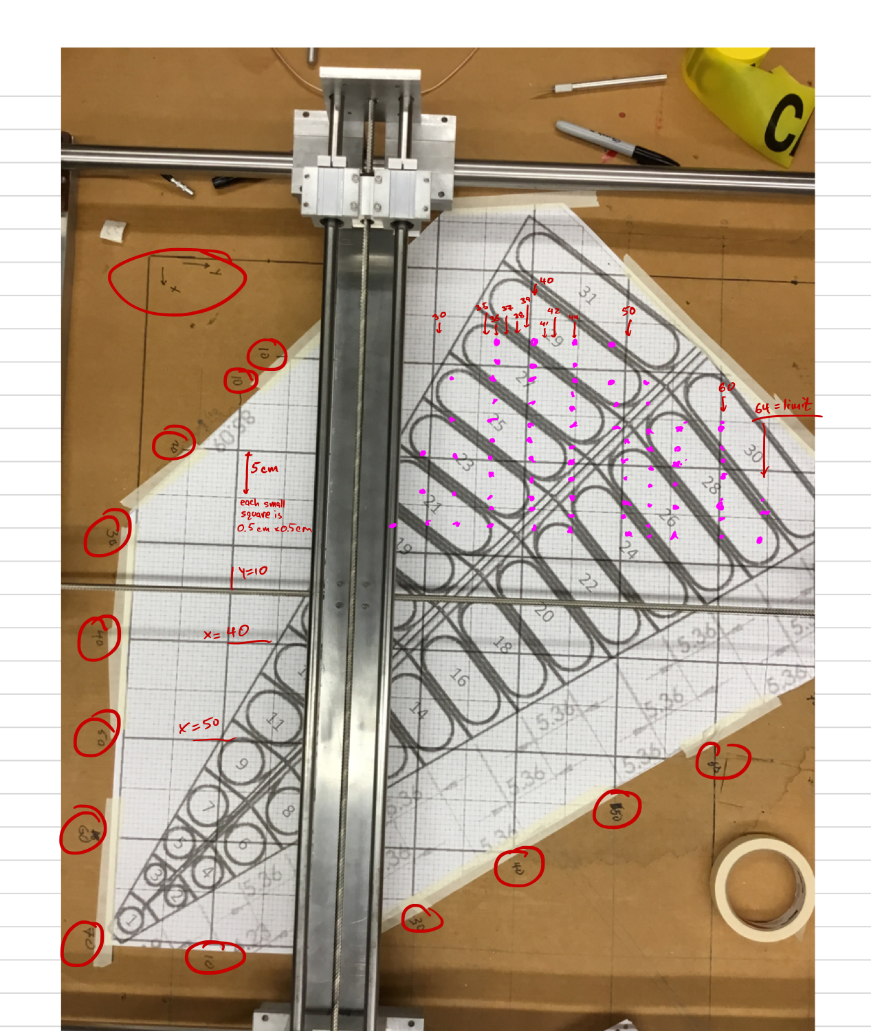
Figure 2 - Pink points show the approximate positions of the source points measured. Notice that the +x direction is downward in this photo, and +y to the right. (Sorry about that.) The mount on which the source sits (source not in photo) is seen at the top of the photo.
With 96 positions to measure, the scan took about 9 hours. The dark current was read for all 31 tiles (and "tile 0" which is the un-connected SiPM) 96x2x10 times (the "x2" is because we measure 10 times with the source under the SS, then 10 times with the source away, for every position).
Below is shown the dark current in uA, as a function of "time", for each of the 32 channels. Sorry about the invisible axis numbers. The dark current is around 1 uA for all.
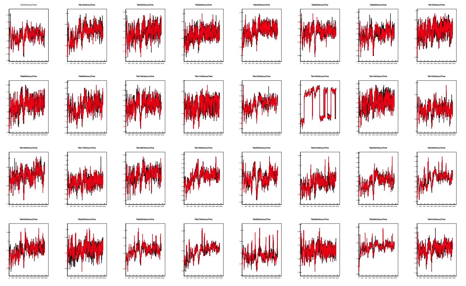
Figure 3 - Dark current as a function of "time", for each of the 32 channels. "Tile 0" in the upper left, is the unconnected SiPM. When the Sr source is away from the SS, the current is drawn as black. When it is under the SS, it is drawn as red. Measurements here are over about 9 hours.
Figure 3 shows that the dark current varies significantly over the course of an hour or so. In fact, several of the SiPMs show a drop in dark current at the same time, in about the middle of the period. The cause for this is unknown. Also, the dark current for Tile 13 has several large jumps, jumping to/from 1.3 to 1.6 uA. The cause of this is also unknown.
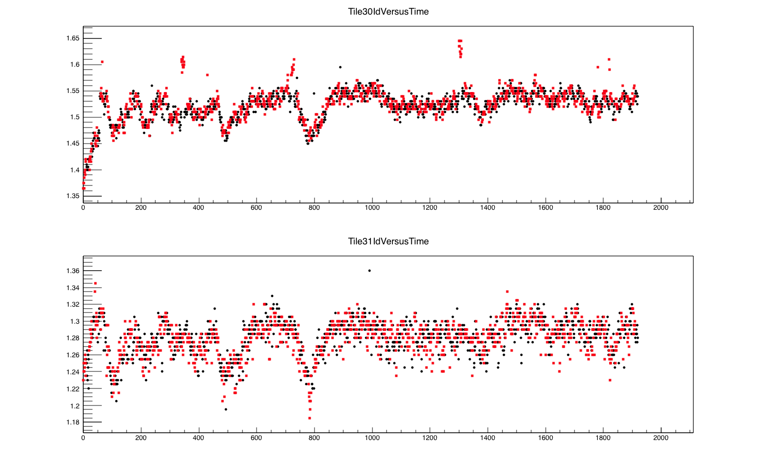
Figure 4 - Strip chart of dark current for Tiles 30 and 31 over the 9-hour measurement period. y-axis is current, in uA; x is "time." Black are when the source is away from the SS, and red is when it is under the SS. Times when the source is under TT30 are clear.
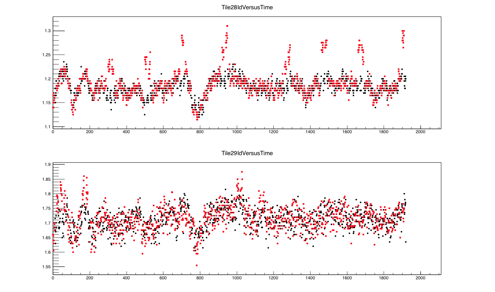
Figure 5 - same as figure 4, but for tiles 28 and 29.
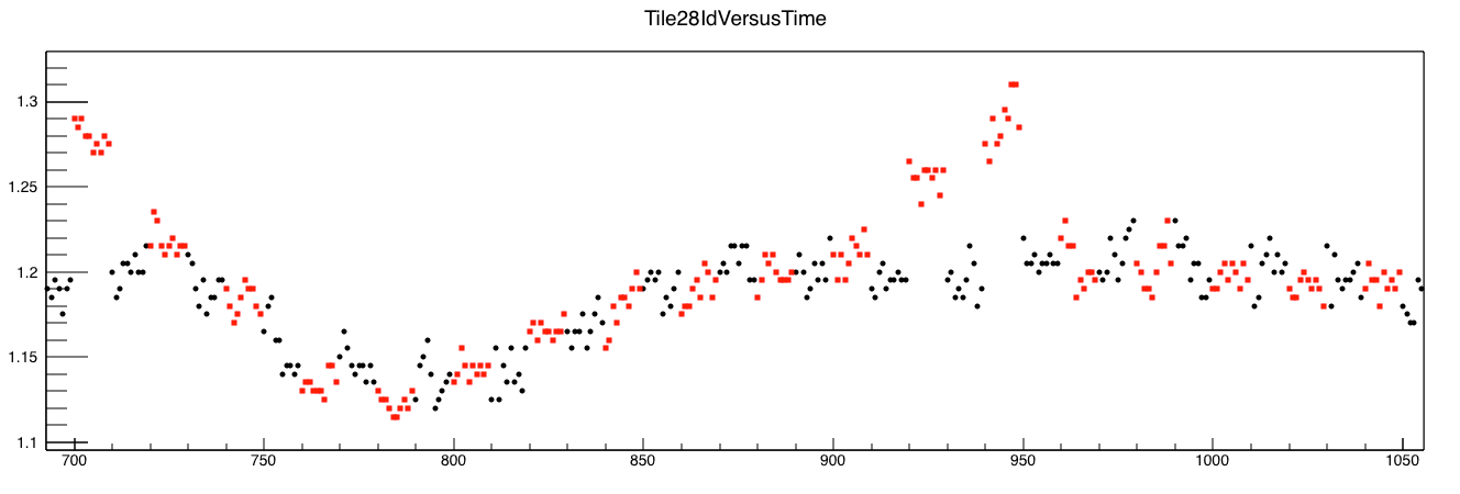
Figure 6 - expanded scale of dark current versus time for tile 28. At several obvious points, the current is higher when the source is under the SS (red points) than when it is not (black points). Clearly, it is important to measure the no-source-present "pedestal" very close in time as the source-present measurement, because dark current varies with time over the course of an hour.
There are two scales to notice in the dark current. First, it varies smoothly (except tile 13) over the course of an hour by about 100 nA. Second, on a sample-by-sample basis, it fluctuates at the 10-nA level. This will set the scale of the changes we will be able to measure.
What is plotted now, is the change in dark current, when the source is placed below a certain position. (The change is relative to the average of the ten measurements that immediately follow the source being moved away again.) If you think about it, you realize that you have to plot a heat map for each tile individually, even if the tile is nowhere near where the source is placed. For this scan, the source is moved over a 24-cm range in x and 20-cm range in y. (Not every point in this rectangular region is sampled, since the supersector is tilted-- see figure 2.)
.png)
Figure 7 - "Heat maps" of tiles 4-7. This is the excess current measured when the source is at position plotted on the axes. (See description above.) These tiles are not in the x-y region of this plot, so one would expect zero excess, except fluctuations. The values fluctuate about zero. (Zero is the middle of the z-scale.)
.png)
Figure 8 - Heat map for tiles 16-19. Our range of sampled points just starts to hit tile 19 (see figure 2), so we see some brightness there, at the level of 80-90 nA.
.png)
Figure 9 - Heat maps for tiles 20-23. TT20 is not hit by the source (see figure 2) so fluctuates about zero. Excess dark current on the scale of 70-90 nA is seen in TT21-23. (Only the edge of TT22 is sampled.)
.png)
Figure 10 - Heat maps for TT24-27. All of these tiles were hit, and see excess dark current at the level 90-120 nA.
.png)
Figure 11 - Heat map for TT28-31. Tile 31 was not sampled by the source, so the excess dark current fluctuates around zero. The other tiles show excess dark current at the 90-120 nA level when the source was below them.
Observations: statistical fluctuations in reported dark current are significant, at the 20-30 nA level, whereas the signal we are looking for is at the 90-nA level. This may be improved (see below). However, I believe we have here an excellent proof of principle.
When the source is held close to the supersector, we have seen about a 200 nA rise in dark current in the close tile. I've described this here. In the current test, in order to hold the SS relatively flat, it is held by a piece of foamboard atop stretched nylon. In this configuration, the increase in dark current is only on order 100 nA.
We are biasing the SiPMs at 56 V (about what we used in the 2017 run). They have been irradiated, so have dark current of about 1.1 uA.
Procedure:
- move the source to some position (x,y) under the supersector, and measure the dark current through the tuff 10 times (I[with])
- move the source away from the supersector and measure the dark current again 10 times (I[without])
- subtract the average of the I[with] from the average of I[without]. It is important to measure I[without] immediately after I[with], because the dark current varies significantly with time, on timescale of tens of minutes.
A full set of plots may be found here
Credit
This scanning set-up is NOT trivial, and I feel the need to identify work done by many individuals over months
- OSU undergraduates Lei Yang (of Yang Solutions, LLC) and Sammy Lisa (of Lisa Innovations, Inc) getting the x-y table to work, with the help of Andrew Kubera and Joey Adams. This took most of the summer for these undergrads and was fun.
- Wanbing He (Fudan U) and Xinyue Ju (USTC) for getting the two processes (driving the xy table and reading currents through the TUFF) to work together and make a root file. This was highly nontrivial and impressive coding.
The setup
Figure 1 - Supersector 06 sits on a foam board atop a stretched nylon netting. The Sr90 source is mounted on an xy table; it is at lower left in the photo. The source is about 1 cm below the supersector when positioned underneath.
Here, I report the first scan of SS06, stepping by 2 cm in x and 4 cm in y. I used 96 positions, focusing on the large-number tiles. The approximate location of the positions sampled is shown below.
Figure 2 - Pink points show the approximate positions of the source points measured. Notice that the +x direction is downward in this photo, and +y to the right. (Sorry about that.) The mount on which the source sits (source not in photo) is seen at the top of the photo.
With 96 positions to measure, the scan took about 9 hours. The dark current was read for all 31 tiles (and "tile 0" which is the un-connected SiPM) 96x2x10 times (the "x2" is because we measure 10 times with the source under the SS, then 10 times with the source away, for every position).
"Strip charts" of the dark current.
Below is shown the dark current in uA, as a function of "time", for each of the 32 channels. Sorry about the invisible axis numbers. The dark current is around 1 uA for all.
Figure 3 - Dark current as a function of "time", for each of the 32 channels. "Tile 0" in the upper left, is the unconnected SiPM. When the Sr source is away from the SS, the current is drawn as black. When it is under the SS, it is drawn as red. Measurements here are over about 9 hours.
Figure 3 shows that the dark current varies significantly over the course of an hour or so. In fact, several of the SiPMs show a drop in dark current at the same time, in about the middle of the period. The cause for this is unknown. Also, the dark current for Tile 13 has several large jumps, jumping to/from 1.3 to 1.6 uA. The cause of this is also unknown.
Figure 4 - Strip chart of dark current for Tiles 30 and 31 over the 9-hour measurement period. y-axis is current, in uA; x is "time." Black are when the source is away from the SS, and red is when it is under the SS. Times when the source is under TT30 are clear.
Figure 5 - same as figure 4, but for tiles 28 and 29.
Figure 6 - expanded scale of dark current versus time for tile 28. At several obvious points, the current is higher when the source is under the SS (red points) than when it is not (black points). Clearly, it is important to measure the no-source-present "pedestal" very close in time as the source-present measurement, because dark current varies with time over the course of an hour.
There are two scales to notice in the dark current. First, it varies smoothly (except tile 13) over the course of an hour by about 100 nA. Second, on a sample-by-sample basis, it fluctuates at the 10-nA level. This will set the scale of the changes we will be able to measure.
First coarse heat maps
What is plotted now, is the change in dark current, when the source is placed below a certain position. (The change is relative to the average of the ten measurements that immediately follow the source being moved away again.) If you think about it, you realize that you have to plot a heat map for each tile individually, even if the tile is nowhere near where the source is placed. For this scan, the source is moved over a 24-cm range in x and 20-cm range in y. (Not every point in this rectangular region is sampled, since the supersector is tilted-- see figure 2.)
Figure 7 - "Heat maps" of tiles 4-7. This is the excess current measured when the source is at position plotted on the axes. (See description above.) These tiles are not in the x-y region of this plot, so one would expect zero excess, except fluctuations. The values fluctuate about zero. (Zero is the middle of the z-scale.)
Figure 8 - Heat map for tiles 16-19. Our range of sampled points just starts to hit tile 19 (see figure 2), so we see some brightness there, at the level of 80-90 nA.
Figure 9 - Heat maps for tiles 20-23. TT20 is not hit by the source (see figure 2) so fluctuates about zero. Excess dark current on the scale of 70-90 nA is seen in TT21-23. (Only the edge of TT22 is sampled.)
Figure 10 - Heat maps for TT24-27. All of these tiles were hit, and see excess dark current at the level 90-120 nA.
Figure 11 - Heat map for TT28-31. Tile 31 was not sampled by the source, so the excess dark current fluctuates around zero. The other tiles show excess dark current at the 90-120 nA level when the source was below them.
Observations: statistical fluctuations in reported dark current are significant, at the 20-30 nA level, whereas the signal we are looking for is at the 90-nA level. This may be improved (see below). However, I believe we have here an excellent proof of principle.
Next steps
- When the source was held, by hand, beneath a supersector, we had seen a 200-nA increase in dark current. In the present arrangement, it is more like 100 nA. This may be due to the foam board on which the detector sits. It is there to increase flatness-- the nylon netting bows too much if the SS sits directly on it. We will probably have to fully support most of the SS on a thick surface, leaving the part to be scanned unsupported. This should be straightforward (though there are mechanical issues, making sure the source gets close enough to the exposed part of the SS, while not banging into the support on the other part).
- It may be possible to get a ~700-uCi source, 3.5x stronger than the present one. This would certainly help us get above fluctuations.
- Reading out more than 10 times per sample would decrease statistical fluctuations in the average, though it goes at sqrt(N), and time is a consideration.
- To get more serious about this, we want a good way to do alignment. (That said, you can maybe kind of align "after the fact," with the data itself, if the sampling resolution is good enough.)
- To look at cross-talk, we will look at correlations in the heat map. I.e. if tile 21 shows excess current when the source is at a given position, does tile 22 see it, too? When we are close to the edge, though, the spread in the source emission is relevant. We need to look at this. Probably most meaningful is to look at such correlations when the source is not near the edge in question.
»
- lisa's blog
- Login or register to post comments