2D Bose-Einstein correlation function in LCMS
Updated on Thu, 2019-04-04 10:37. Originally created by mcsanad on 2019-04-02 07:10.
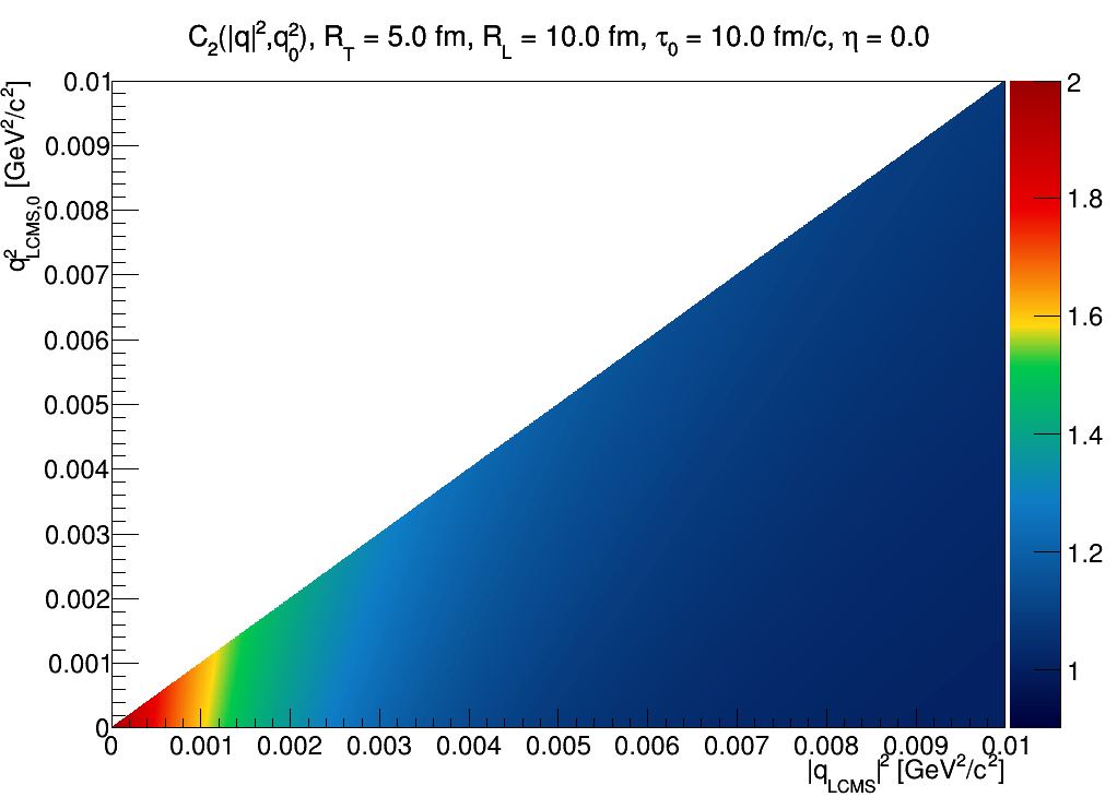


One can immediately see that at midrapidity, dependence is (almost) only on |q|, not on q0, hence also not on qinv2=|q|2-q02, constant values of which are parallel to the diagonal of this plot, and qinv=0 is represented by the diagonal.
For other source parameters (note that RL only matters if |η|>0; and η only matters if RL≠RT) the plot changes slightly, but not dramatically:

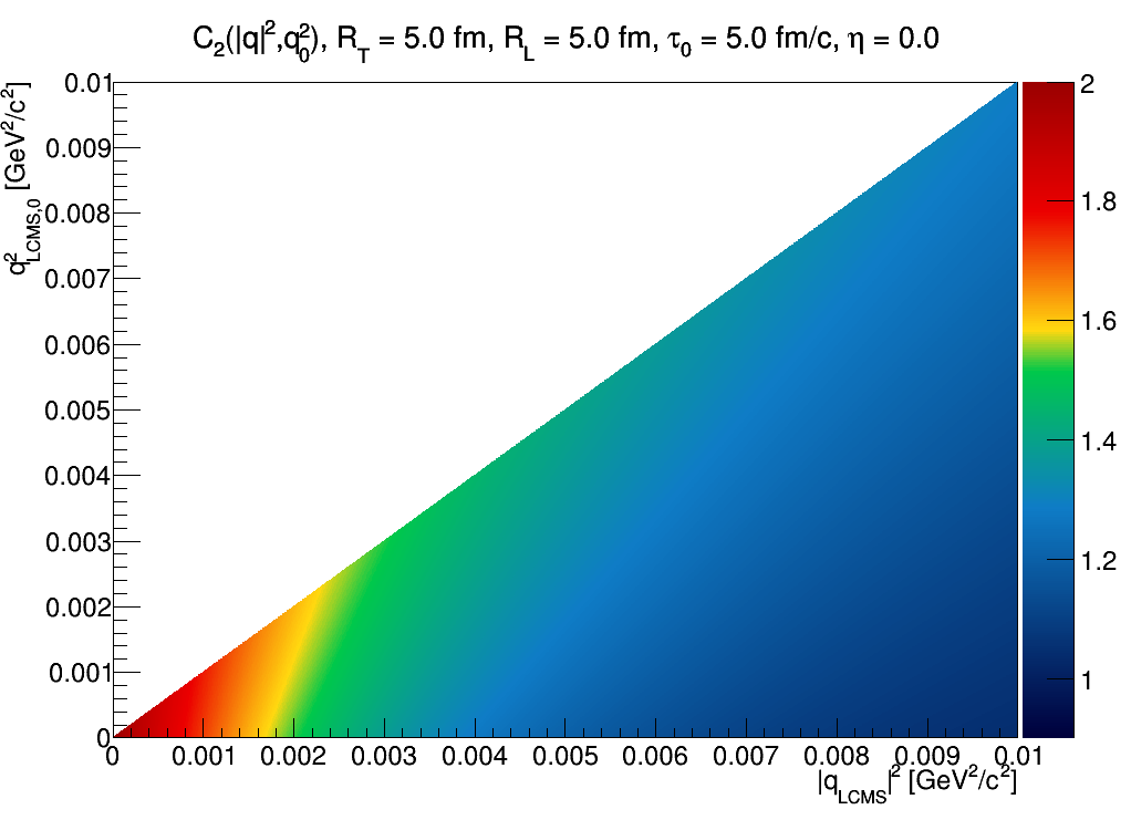
I.e. the peak is less tilted towards the diagonal if emission time is larger than the spatial dimensions.
double qT2 = q2/cosh(eta)/cosh(eta);
double qL2 = q2*tanh(eta)*tanh(eta);
double AT = (RT2+tau02)*RT2*tau02/((RT2+tau02)*(RT2+tau02)+tau02*RT2*RT2*q02);
double AL = (RL2+tau02)*RL2*tau02/((RL2+tau02)*(RL2+tau02)+tau02*RL2*RL2*q02);
double C2 = 1 + exp(-qT2*AT-qL2*AL);
if(q02>q2) C2 = 0;
Such a source is expected in e+e- collisions where multiple jets were created - but our case seems to be very different from this.
Calculation
We start from a spatial Gaussian in the LCMS frame (where there is one transverse and one longitudinal size): exp(-(rx2+ry2)/2RT2-rz2/2RL2), and a Dirac delta in coordinate proper time: delta(τ-τ0). Then we perform a Fourier transformation (by doing a second order expansion in the exponent, needed because of the t→τ transition. The absolute square of this (imaginary) quantity is the correlation function minus unity, so we add one, and obtain the result for the Bose-Einstein correlation function. Since I don't know as of now how to include complicated formulas to this webpage, I refrain from doing so.Results
Our correlation function result is given as a function of qT,qL,q0, so we first introduce pair pseudorapidity η, and then we can express our results as a function of |q|2 and q02. Let us show results for τ0=RL>RT:One can immediately see that at midrapidity, dependence is (almost) only on |q|, not on q0, hence also not on qinv2=|q|2-q02, constant values of which are parallel to the diagonal of this plot, and qinv=0 is represented by the diagonal.
For other source parameters (note that RL only matters if |η|>0; and η only matters if RL≠RT) the plot changes slightly, but not dramatically:
I.e. the peak is less tilted towards the diagonal if emission time is larger than the spatial dimensions.
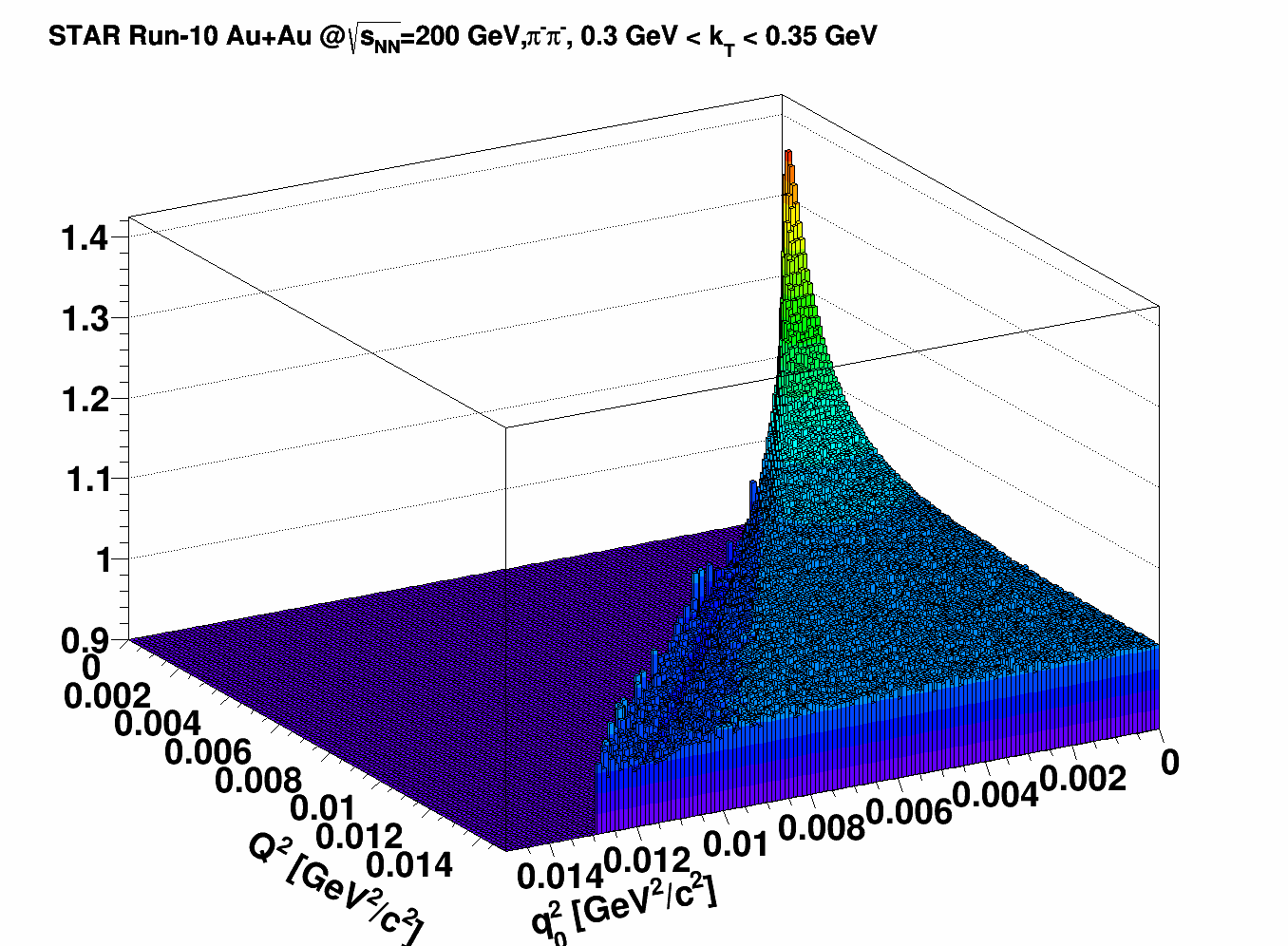
Data
The data show striking similarity with the above toy model:
Appendix
For those interested, here is the analytically expressable result for the Gaussian case, to be used e.g. in ROOT, assuming q2 and q02 are the above variables, eta the pair pseudorapidity, while RT2, RL2 and tau0 are the source parameters (squared, and in c2/GeV2 units, i.e. divided by hbarc2).double qT2 = q2/cosh(eta)/cosh(eta);
double qL2 = q2*tanh(eta)*tanh(eta);
double AT = (RT2+tau02)*RT2*tau02/((RT2+tau02)*(RT2+tau02)+tau02*RT2*RT2*q02);
double AL = (RL2+tau02)*RL2*tau02/((RL2+tau02)*(RL2+tau02)+tau02*RL2*RL2*q02);
double C2 = 1 + exp(-qT2*AT-qL2*AL);
if(q02>q2) C2 = 0;
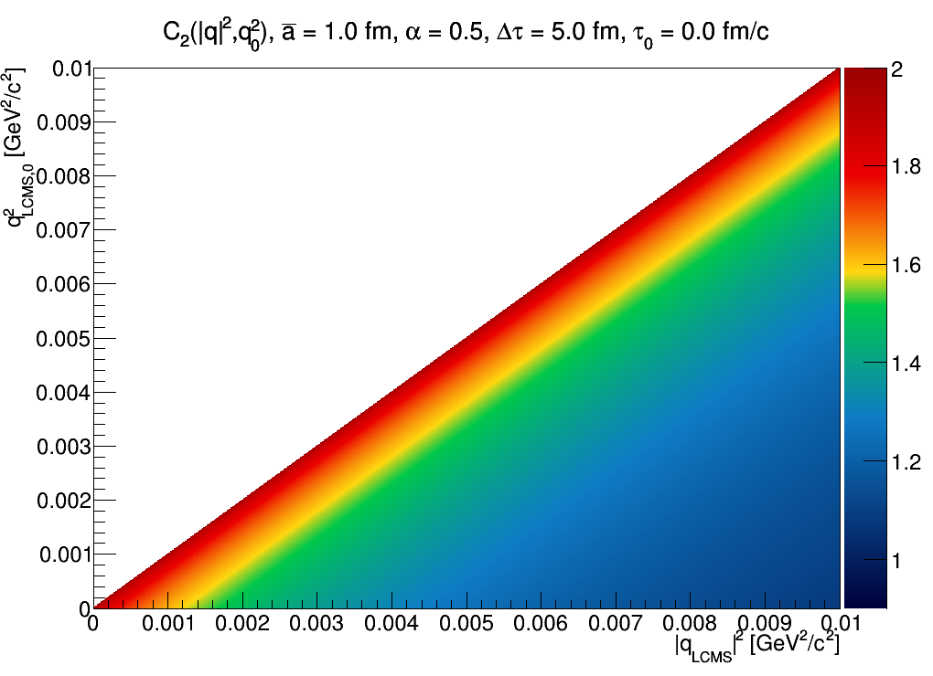
Sidenote
Let us, contrary to the above, take a source wich may be characterized by a maximal emission point proportional to momentum and proper-time, i.e. xbar = a*τ*p, and an emission distribution in proper time H(τ) being a one-sided Lévy distribution. This now not the spatial emission probability density, but the one in proper time. This source results in a correlation function where qinv appears as the only momentum-difference carrying term. Hence, the correlation function will look like:Such a source is expected in e+e- collisions where multiple jets were created - but our case seems to be very different from this.
»
- mcsanad's blog
- Login or register to post comments