vernier scan fit implementation
My code as written is producing unrealistically small cross sections, so I wanted to explicitly write out the way I'm performing the fit:
The input to the code is a histogram of the number of events in each one-second bin of the run, and one of the following sets of arrays and values:
| 10103044 | Ny=10039.98 | kB=107 |
| Nb=10505.05 | Tmax=1400 | |
| timediff | x | y |
| 00 | 0.0 | 0 |
| 36 | 0.15 | 0 |
| 37 | 0.30 | 0 |
| 36 | 0.45 | 0 |
| 36 | 0.60 | 0 |
| 36 | 0.75 | 0 |
| 36 | 0.90 | 0 |
| 41 | 0.0 | 0 |
| 36 | -0.15 | 0 |
| 36 | -0.30 | 0 |
| 36 | -0.45 | 0 |
| 36 | -0.60 | 0 |
| 36 | -0.75 | 0 |
| 36 | -0.90 | 0 |
| 41 | 0 | 0 |
| 31 | 0 | 0 |
| 36 | 0 | 0.15 |
| 35 | 0 | 0.30 |
| 36 | 0 | 0.45 |
| 36 | 0 | 0.60 |
| 36 | 0 | 0.75 |
| 36 | 0 | 0.90 |
| 41 | 0 | 0 |
| 37 | 0 | -0.15 |
| 36 | 0 | -0.30 |
| 36 | 0 | -0.45 |
| 36 | 0 | -0.60 |
| 36 | 0 | -0.75 |
| 36 | 0 | -0.90 |
| 41 | 0 | 0 |
| 10097097 | Ny=10274.33 | kB=107 |
| Nb=11349.49 | Tmax=1220 | |
| timediff | x | y |
| 00 | 0.0 | 0 |
| 35 | 0.10 | 0 |
| 35 | 0.20 | 0 |
| 37 | 0.35 | 0 |
| 36 | 0.50 | 0 |
| 37 | 0.75 | 0 |
| 37 | 1.0 | 0 |
| 41 | 0.0 | 0 |
| 35 | -0.10 | 0 |
| 35 | -0.20 | 0 |
| 37 | -0.35 | 0 |
| 35 | -0.50 | 0 |
| 37 | -0.75 | 0 |
| 37 | -1.0 | 0 |
| 42 | 0 | 0 |
| 31 | 0 | 0 |
| 35 | 0 | 0.10 |
| 36 | 0 | 0.20 |
| 36 | 0 | 0.35 |
| 35 | 0 | 0.50 |
| 37 | 0 | 0.75 |
| 38 | 0 | 1.0 |
| 41 | 0 | 0 |
| 35 | 0 | -0.10 |
| 35 | 0 | -0.20 |
| 35 | 0 | -0.35 |
| 36 | 0 | -0.50 |
| 37 | 0 | -0.75 |
| 37 | 0 | -1.0 |
| 42 | 0 | 0 |
timediff (s) - the time between the timestamp of the end of the previous step, and the timestamp of the end of the current step
x (mm) - the position of the beam in the x direction
y (mm) - the position of the beam in the y direction
Nb (10^9 Ions) - the number of ions in the blue beam
Ny (10^9 Ions) - the number of ions in the yellow beam
kB - the number of bunches per beam
Tmax (s) - Roughly the end of the run, used to keep the code that finds the offset between T=0 for the run and T=0 for the tables above from running off to infinity.
These tables are derived from information Angelika gave me (I'll create a small blog page for just that raw information, and hopefully link it here).
Determining the offset:
I create a new array, "timestamp" that sums all the timediffs up to i to get the total time since the start of the run until the ith step. I add to this a proposed offset (in seconds). I then check the difference in rate across each of the four largest steps (1,-1 to 0; .9,-.9 to 0 depending on the run), which occur at the end of the (c counting) 6,13,21, and 28th bin. I sum the two seconds following each of the timestamps, then subtract from that the two seconds before each one, and choose the offset that maximizes this value.
Rebinning the rate histogram:
Using the best offset from the previous, I fill a new histogram indexed by the steps of the vernier scan by summing across 28 seconds of the rate histogram, starting 30 seconds before the timestamp and ending 2 seconds before it to ensure I don't integrate over the period when the beam is moving.
Fitting the new histogram:
I create a TF1 with a special function defined:
Double_t gaus_stepping(Double_t *v, Double_t *par)
{
  Double_t skfNN=par[0]*frequency*Nbunches*Nblue*Nyellow/10000000;
  Double_t sx2=par[1];//sigx1*sigx1+sigx2*sigx2; //milimeters^2
  Double_t sy2=par[2];//sigy1*sigy1+sigy2*sigy2; //milimeters^2
  Double_t background=par[3];
  Int_t step=v[0];
  if (step>29) return 0;
  Double_t dx=x [step];
  Double_t dy=y [step];
  if ((sx2*sy2)<0.00000001) return 0;
  Double_t sL= skfNN/(2*TMath::Pi()*sqrt(sx2*sy2));
  Double_t val=sL*exp(-dx*dx/(2*sx2))*exp(-dy*dy/(2*sy2));
  return (val+background)*integration_width;
}
frequency (MHz) - a constant 9.383/120.0
par[0] (nb) - the cross section for the event
par[1] (mm^2) - the sum of the squares of the widths of the two beams in the x direction.
par[2] (mm^2) - the sum of the squares of the widths of the two beams in the y direction.
par[3] - the rate of background events.
skfNN (MHz*cb*10^9*10^9=Hz*b*10^22=Hz*cm^2/10^2=Hz*mm^2) - since I input the cross section in nanobarns, I need to divide by 10^7 (that is, cb/nb)
I take this value and compute the full-on luminosity (if the position were x=y=0):
sL (Hz) - skfNN/2*pi*sqrt(sx^2)sqrt(sy^2)
val (Hz) - the two exponentials account for the offset from full-on in each direction, using the distance we get from the tables above, for a given time bin.
We return the value of the itneracting beams plus an assumed flat background, multiplied by the 28 seconds we integrated over to populate each bin.
The problem is that this approach yields values that are far too small:
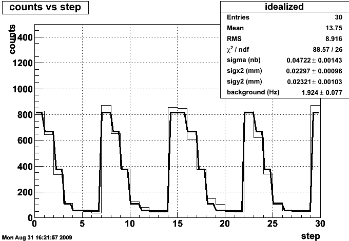
This value, 40 picobarns, can be disproven by eye - we took easily over 10^5 BHT3 events, and we certainly didn't have 2500 inverse picobarns delivered to the experiment.
- rcorliss's blog
- Login or register to post comments