In all upsilon analyses (pp 2006, AuAu 2007, dAu 2008, pp 2009, AuAu 2010) it is necessary to match candidate tracks with BEMC clusters/towers that could have fired the trigger.  This removes what we call "random benefit" of forming a potential candidate that could not be triggered on and thus won't be accounted for in the calculated efficiency.

The way in which tracks were matched to clusters was to look at the distance in eta-phi space between the cluster center and the point on the BEMC that the track in question extrapolates to.  This distance we gave the label R, where R = sqrt((delta eta)^2+(delta phi)^2).  The weighted average for phi (or eta) was calculated as:

phi ave = (phi1*E1+phi2*E2+phi3*E3)/(E1+E2+E3).

The problem is that if a cluster is near pi (-pi) calculating the average could result in a value anywhere between -pi and pi, which means that tracks that should have matched, will fail, since the track phi is calculated directly.

This method was used in in the published pp 2006 cross-section calculation.  However, since this method was used both in the MC efficiency calculation and in the data, the effect should cancel.  Basically, this is like changing the acceptance of our detector a little around phi = pi.  So, our statistical  error bars should be a little bit smaller, but given the high efficiency of the matching to begin with (~92%) the reduction in the statistical error bars would be small, at most 8%. 

From this point on, the phi average will be calculated by:

phi ave = atan2( (E1*sin(phi1) + E2*sin(phi2) + E3*sin(phi3))/Ecluster,
  (E1*cos(phi1) + E2*cos(phi2) + E3*cos(phi3))/Ecluster

Using the 2010 single electron embedding, assuming an electron momentum distribution weighted by what we'd expect from upsilons, I generated the following graphs using the "old" way.

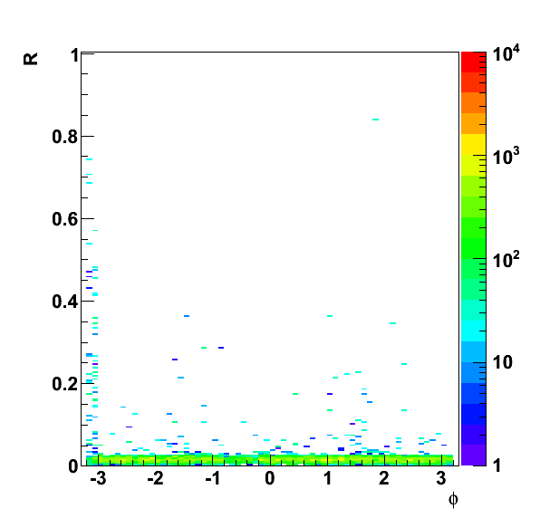
Figure 1. R versus phi for electrons that satify L0 trigger conditions, are reconstructed and pass track quality cuts.  We can see the issue at phi = -pi,pi.

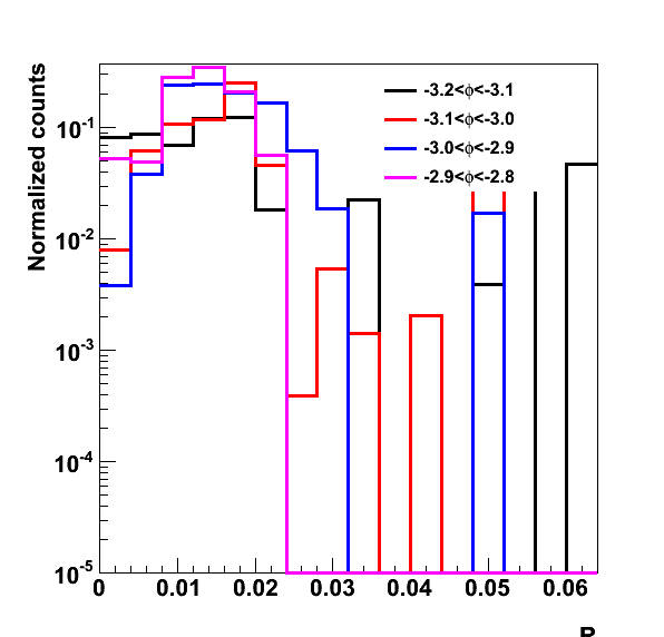
Figure 2.  R for select bins in phi.  I have normalized these distributions by dividing by the number of counts simply to graph them together.  From Figure 1, we can see that in the range |phi| < 3 the value is relatively constant, thought there does seem to be a slight increase at +/- pi/2. 

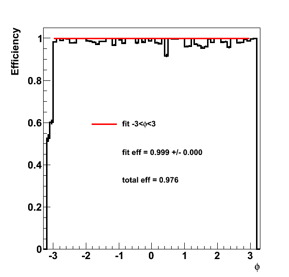
Figure 3.  Efficiency for the R cut vs phi.  The error bars aren't quite right as I'd have to take into account the weighting better....  In any case, for this, the total efficiency is calculated from -pi to pi, and the fit efficiency is from -3 to 3.  Not particularly happy with this fit as it seems high to my eyes, probably because the error bar is off.  But either way, the numbers won't change too much.  Also note that the efficiency is higher than the 2006 quoted value.  This is probably due to the removal of the inner track material, though I haven't extensively studdied this.  Also, multiplicity has a reasonable effect so these were from those events with refMult<100 to see if we get the same values as for pp.