In order to better understand how we should run for next years BES running, I looked at the 27 GeV data (pico Dst, fastoffline).

The vertex distribution is below.

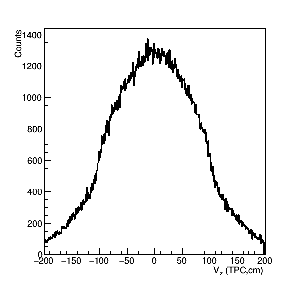
Figure 1: Vz distribution for the 27 GeV data.  We can see here that one issue was a the large size of the beam extended the distribution beyond a nice window (say |Vz| < 80 ?  I forget what the goal was)

The question is, could we do better with the Epd acting as a tighter trigger than the bbc?  (Especially as we go down in energy, the greater acceptance compared to the vpd could help.)

This requires that we slew correct the tiles.  Looking at a single tile:

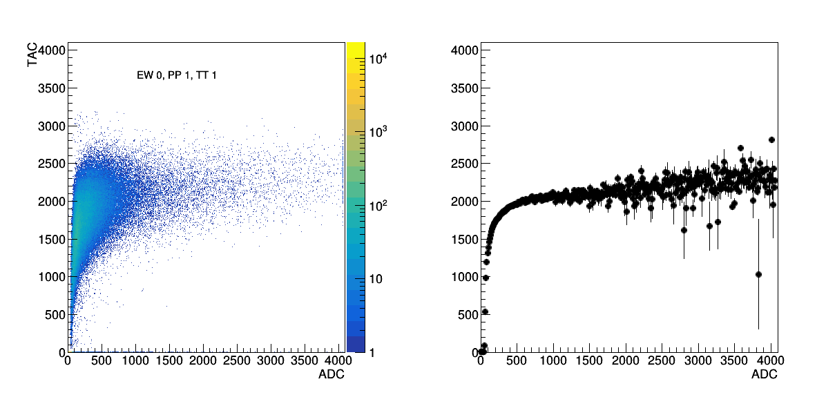
Figure 2: ADC vs TAC for East position 1 tile 1 on the left, with the profile on the right.

From Figure 2 we see that the swing vs ADC is quite large, especially at low ADC.  Both TAC and ADC had a max of 4095.  It should be noted that the mip peak was set around 160 for these inner tiles.  If you want to see this distribution for all files, it can be found at: drupal.star.bnl.gov/STAR/system/files/ADCTAC_27GeVFull_11112018.pdf

Zooming in:

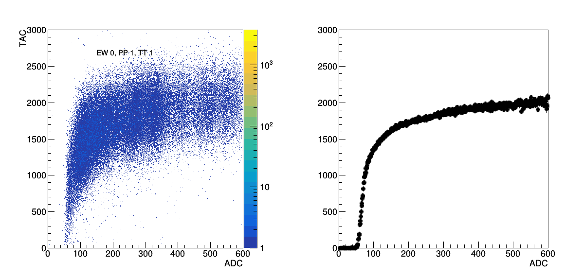
Figure 3: Zoomed in version of Figure 2.

One of the issues that I ran into while trying to apply the slew correction, was that it can only be applied in 8 bins in ADC (and these must be the same for all) and the correction range goes from -255 to 255.  From Figure 2 and 3, we see our dynamic range is much greater than this.  This means it will be impossible to fully correct, and that we should concentrate on the higher end where things are more stable.  

The bins I had chosen were: {0, 75, 100, 125, 150, 175, 200, 500, 4095};
Unfortunately, most of the range was in this area of where it is irrelevant.  (It should be noted that we must start at 0 and end at 4095, though the zero is not required in the slew correction file itself.)

Without corrections, we can count how often a particular channel was the fastest TAC on the east or west.  (Here I required a minimum adc of 15, and that both the east and west had at least 1 tile with an in-time tac.)

Comparing the profiles of a number tiles together, we see:

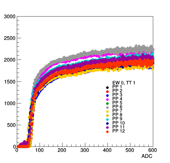
Figure 4: Profiles of a number of different channels linked to the same side and tile (so the multi-mip hit probability would be the same).  We see that there is quite a spread.  If you want to see comparisons of all the others, look at: drupal.star.bnl.gov/STAR/system/files/CompareProfile_All_27GeV_11112018.pdf

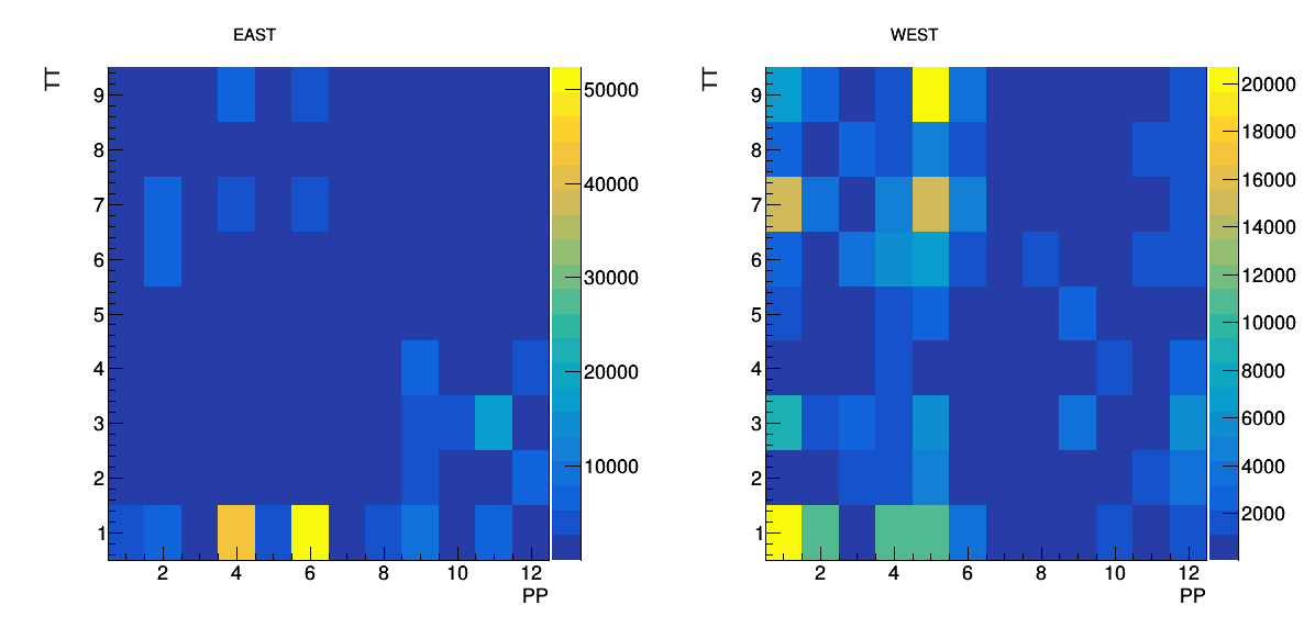
Figure 5: Number of times a given tile was the fastest tile in an event.  We see that we're really being driven by PP6 TT1 on the East and PP1TT1, PP5TT9 on the west.

Comparing the two with the most egregious spread:

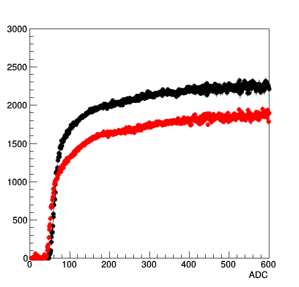
Figure 6:  Comparison of East Tile 1 for PP 6 in black and PP 7 in red.  We can see why Tile 1 PP 6 fires the most often of all the tiles on the east.

We can look at the east fastest versus west fasted TAC, and compare this to the TPC Vz (here I'm making no quality selections on the latter for the moment).  It should be noted that the relationship between TAC and time is 15.6 ps/ch.

If we plot the fast east vs west and compare this to the vertex position, we get:

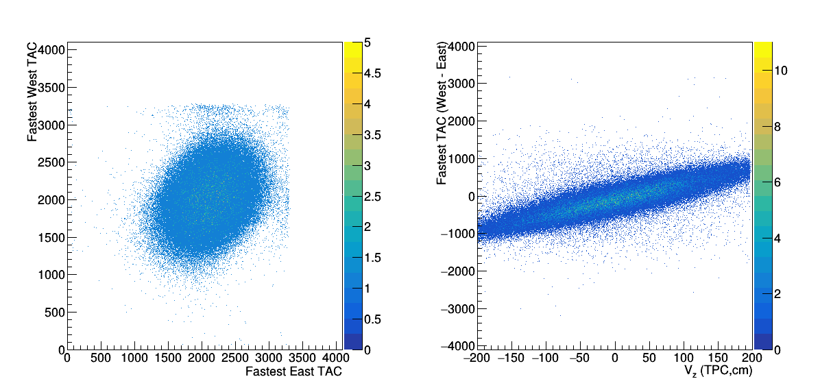
Figure 7: On the left is the Fastest TAC East vs Fastest TAC West.  We see a nice correlation between the two, which would be expected as the Vz distribution is centered (if broadly) on Vz = 0.  On the right is the West - East difference in TAC vs TPC Vz.  

This is actually not all that bad, one would expect the value on the edge to be ~ -850 on the east, and we know from the previous study that we're more fooled by outliers...  I guess one issue before was the beam satellites at the higher energies, because then one can have these very different distributions.

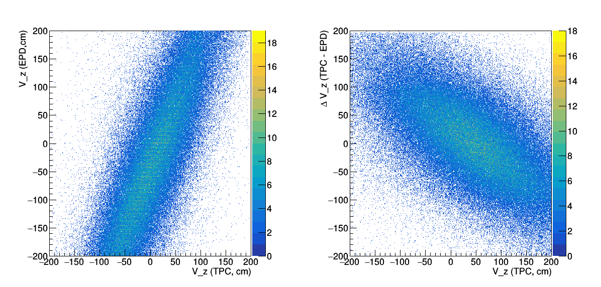
Figure 8: On the left is the TPC Vz vs the EPD Vz on the right is the difference in Vz (TPC - EPD) vs the TPC Vz.  As expected, pulled by the tails.  But this does mean the resolution will be terrible (though not offset).

So next we should figure out what our range should be...  I will do this by summing up all of the 2D histograms, and then setting the lower range to be where the line at ADC = 160 (1 MIP) would cross the lower end.  

This results in:

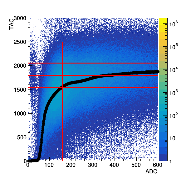
Figure 9: Sum total of all ADC-TAC files, with the black points as the profile.  The vertical red line shows where the MIP peak is, the three horizontal lines show the range of the correction factor.

This means we will try to center the TAC values at TAC = 1800.  This also gives us the bin edges of:
bin = {0,150,225,300,375,450,525,600,4095}

where I shifted the second bin line to make a nicer number.

This doesn't turn out to be the best option in the whole world....  A good example is EW0PP6TT1, which was our East side culprit before.

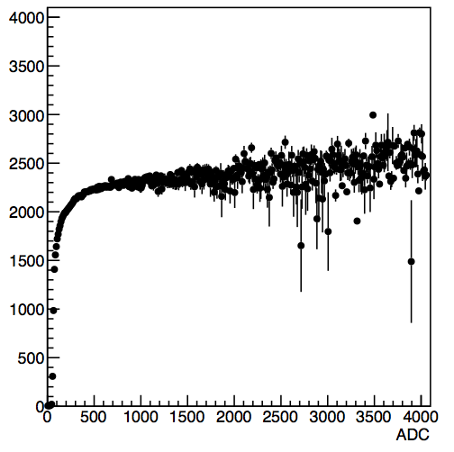
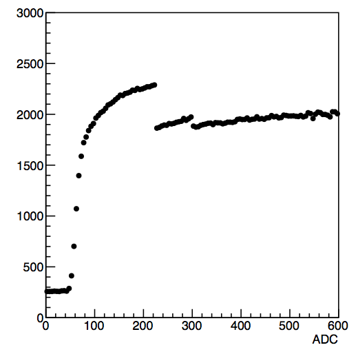
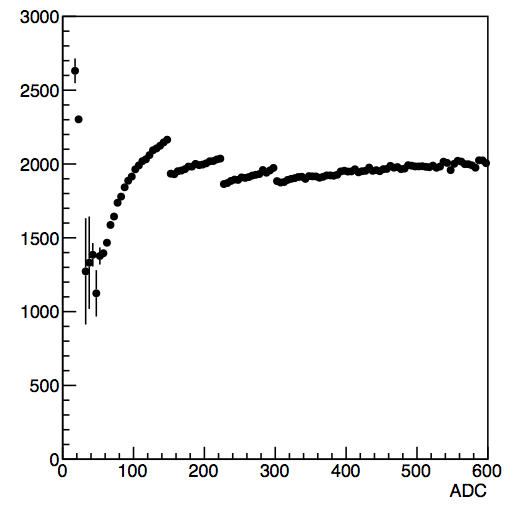
Figure 10: EW0PP6TT1.  The right plot is the uncorrected data.  The middle is simply correcting each of the bins by the bin average.  The right plot was after I changed the correction value of the second bin from 255 to 0, decreasing it.  (For the right plot I also threw out TAC < 10 events).

Ok.  Perhaps this should have been obvious to me, but I want to correct based on the high edge of the bin and not the center.  I will do this, look at the distributions and then look at what happens when I require ADC > 160.  (This is what I ended up doing for the resolution study.)

Incidentally, it did help a bit, but not perfectly:

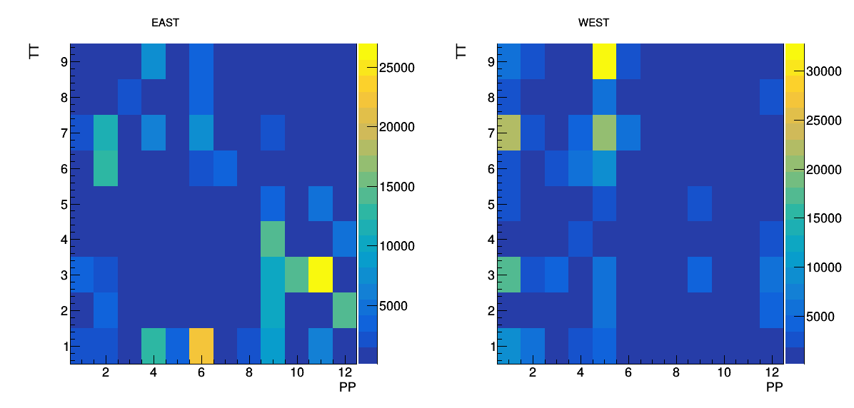
Figure 11: Fastest TAC ID East vs West after the correction and after I fiddled with EW0PP6TT1.

With this other method, I get something more like:

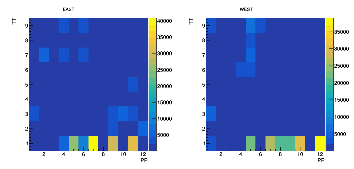
Figure 12: Fastest TAC ID East vs West after the correction where the factor comes from the highest ADC in the bin.

Chatted with Hank, there is a way to do a TAC offset!  Ok, I had recalled Akio saying something about this.  For now (since this will be discussed Tuesday) I will dummy it in....  I'm also going to aim for TAC = 2000 instead of 1800.  

This is starting to look a little more promising, now if we compare the profiles:

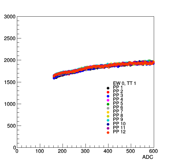
Figure 13: TAC Profiles vs ADC with TAC offset.

If you want to see all the different distributions, look at: drupal.star.bnl.gov/STAR/system/files/ADCTAC_27GeVFull_11112018_tacoffset.pdf

Interestingly enough, if we look at the ids of the fastest tac:

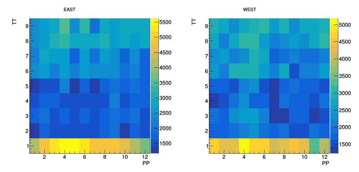
Figure 14: ID of the tile that was the fast TAC after applying a TAC offset.  Note the scale difference from the previous ones!

Then we can apply the slew correction:

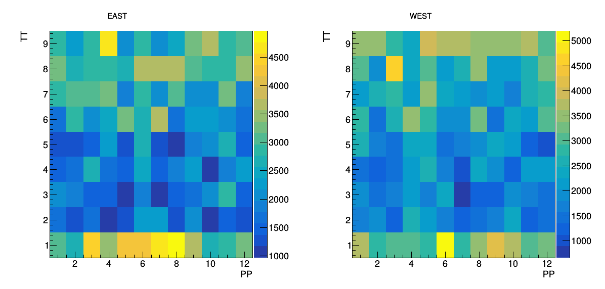
Figure 15: ID of the tile that was the fast TAC after applying a TAC offset and a slew correction.

It's interesting to see that tiles 1, 7-9 seem to be more often selected... I assume it's a combo of spectators in 1 and participants in 7+.  Perhaps some masking and more careful analysis will help (for instance, leaving out tile 1).

But lets see what this looks like:

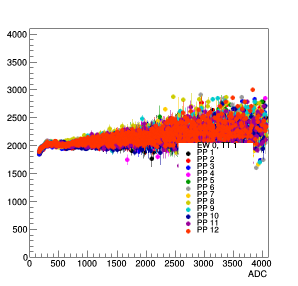
Figure 16: Looks pretty flat ... (TAC vs ADC), so this has mostly done a reasonable job.

If anyone wants to flip through all the pdfs:
profiles at: drupal.star.bnl.gov/STAR/system/files/CompareProfile_All_27GeV_11112018_tacoffsetslew.pdf
everything at: drupal.star.bnl.gov/STAR/system/files/ADCTAC_27GeVFull_11112018_tacoffsetslew.pdf

But what about picking out the vertex?  If we look at the relationship:

Figure 17: Fast TAC East vs West after correction on the left, delta fastest TAC vs Vz.

This looks cleaner than it did....  But I think I should clean up further (last time I removed outliers at the high end but I won't have time tonight) as the slope isn't right, which is what I saw in the earlier analysis prior to removing them.  In any case, if I make a selection to try to choose |Vz| < 50, let's see how that works.  First the vertex comparison:

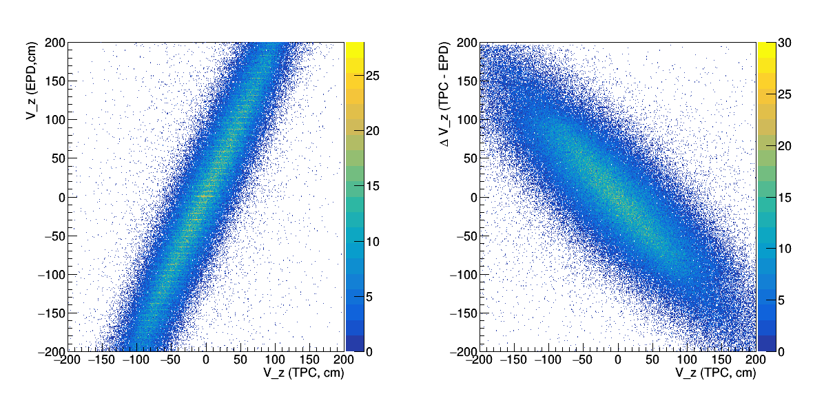
Figure 18: Vz epd vs TPC...  As noted, slope isn't quite right.  

But let's try to "trigger" on events regardless.  So first we can look at the delta TAC for |Vz|<50:

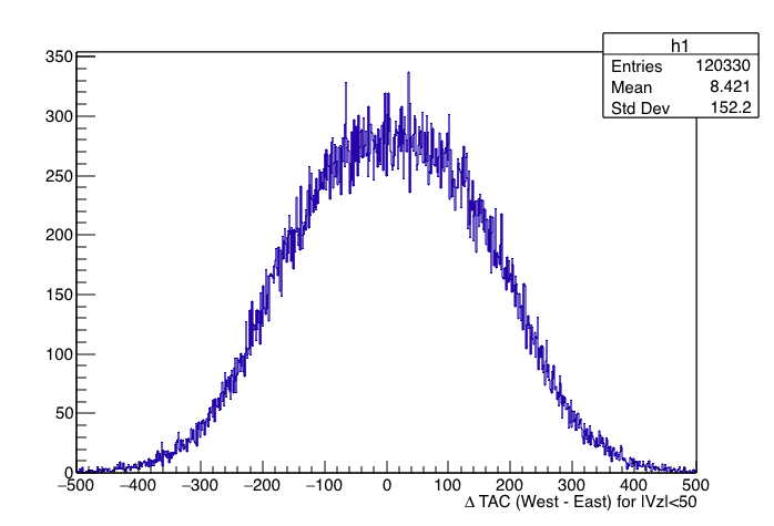
Figure 19: Delta TAC after offset and slew correction for |Vz| <50.  Using a 2 sigma approach, I will select events with |Delta TAC| < 300, which should be about 95% of all events with vertices in that range.

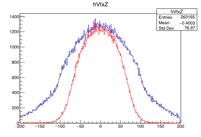
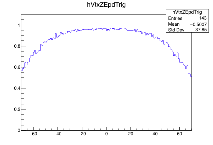
Figure 20: Vz of all events in this sample in blue, Vz of the epd triggered events in red.  The ratio of the two is the left plot, we see that between 40 and -40 the efficiency is at about 95%.  Of course, we still have events outside the window, but there is still work to be done.