Executive Summary:

With a crude slew correction, we find that the spatial resolution of the EPD corresponds to 11.8 cm, which corresponds to 11.8/0.03 = 390 ps (0.39 ns) using an average TAC value of the QT32C channels on the East and on the West sides.  There is room for further improvement with a better slew correction.

Figure 0: Difference in vertex Z distribution between the vertex found by the EPD and found using the TPC.  Some cuts have been applied to select good events, to select in-time TPC vertices, to crudely slew correct the EPD.

Details below

We can use the TPC vertex to determine the timing resolution of the EPD vertex, as this will have a much higher spatial resolution (on the um level) which means we are not convoluting the resolution of the secondary detector into the EPD resolution..  The issue is that we need to be able to choose the "in-time" vertex (knowing that many things are not calibrated) or we will get some very weird tails in our distrubionts.  First, let us look at the state of the data from day 107 (picoDst!).

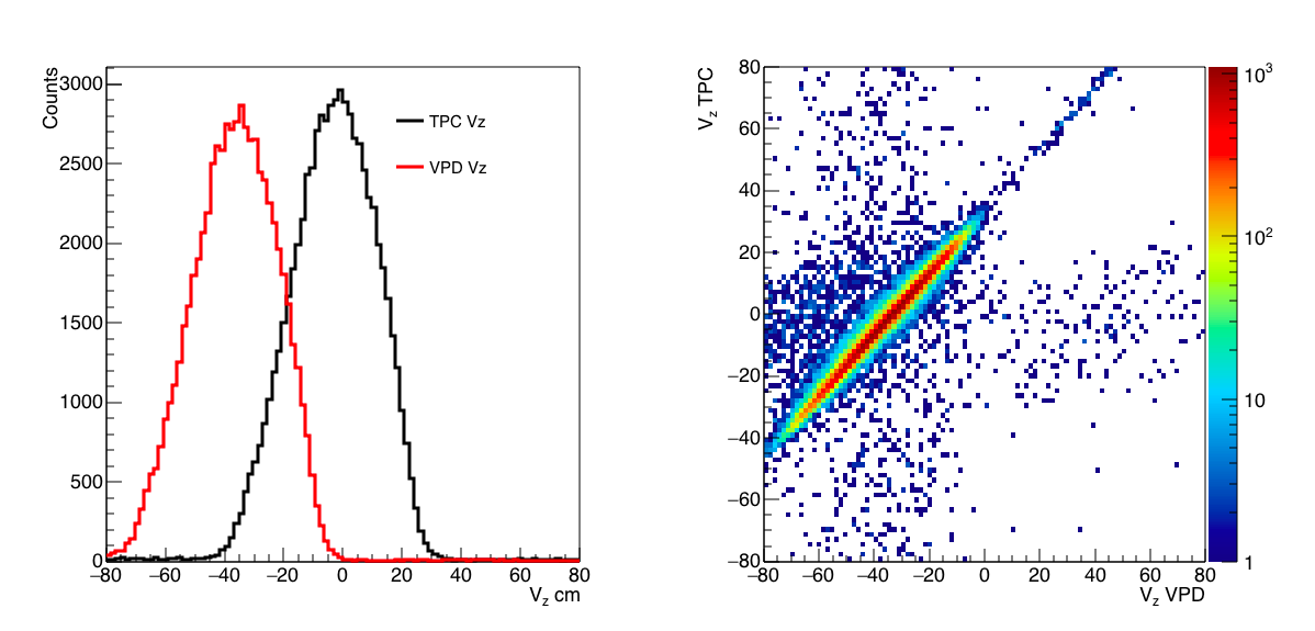
Figure 1: (Left) Vz distributions for the TPC vertex (black) and the VPD vertex (red).  We see here that the VPD Vz would need to be calibrated first.  (Right) Vz TPC vs Vz VPD, here we can see the correlation is tight other than the offset, so we can use the VPD to choose the proper vertex but need to shift the distribution so that the two are peaked at the same place.

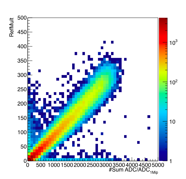
Figure 2: Sum of the ADC/ADC_1Mip distribution versus RefMult from the TPC.

In Figure 2 we can see that the EPD and TPC do mostly agree on the centrality, though there are some out-of-time vertices and pile-up effects that can be seen.  I will clean up this sample prior to using it to QA the TPC vertices.

First, let's see where we are out of the box for the EPD.  The TAC vs ADC distributions (uncorrected) can be seen at:
drupal.star.bnl.gov/STAR/system/files/tac_04182018.pdf

To calculate the vertex, first I found the fastest TAC on the East and West (fastest = largest), and then determined West - East.  I believe that the calculation should be 15.6 ps/ch and that the speed of light moves 0.03 cm/ps.  Using this, I can turn delta TAC into a vertex.

Figure 3: (Left) Fastest TAC East vs West.  (Middle) Fastest TAC East vs West. (Right) First calculation of EPD Vz.

From Figure 3 we see that there is a nice correlation between the East and West, however, the vertex distribution looks odd (one is seeing some sort of integer type issue in the distribution).  I require that the ADC is above threshold for a TAC to count.  I suspect that most of the issue is due to the fact that different tiles level out at different TAC, so without a slewing correction only a few tiles are really determining the Vz position.  I am surprised it is so peaked, though, because the distribution in the middle panel of Figure 3 actually looks somewhat reasonable.

Figure 4: (Left) Comparison of the uncorrected EPD Vz versus the Vz from the TPC. (Right) Comparison of the TAC vs ADC for EW 0 PP1 Tile 3 (black) and Tile 4( red).

Looking at Figure 4 I am obviously wildly off.  We see from the distribution on the right of figure 4 that at the very least a vertical offset is needed.

So first I will do a crude recentering of vpd.  The mean of the Vz VPD distribution is -36.3046 cm and the mean of the Vz TPC distribution is -3.13415.  So I  will calculate a corrected vpd vz as:

VPD Vz Corr = VPD Vz +36.3046 - 3.1345

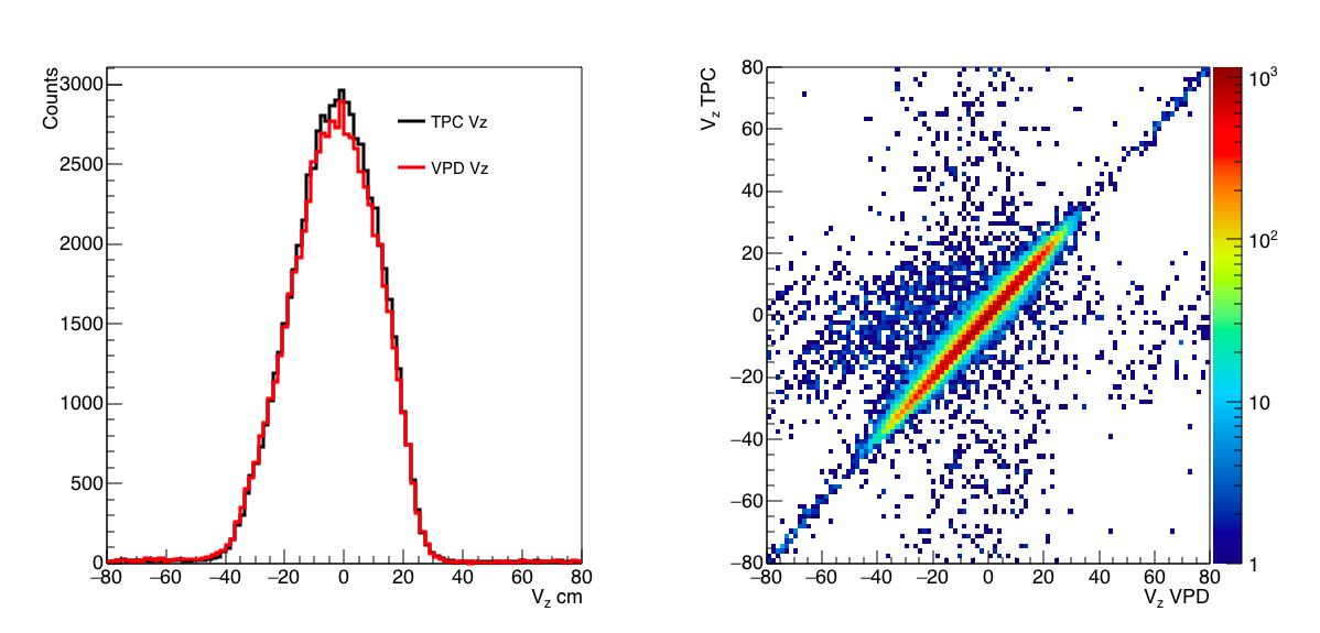
Figure 5: Vertex distributions for the TPC vs VPD Vz after correction. 

From now on this blog, the VPD Vz I refer to will be this corrected VPD Vz.  In order to make things easier, I will now require the following cuts:
|Vz| < 20
|Vpd Vz| < 20
|Vpd Vz - Vz| < 6

The last cut is ~2 sigma cut on the Vpd Vz resolution (3 cm), so we will discard very few real events.  This also centers the distributions in STAR, which should make things easier.

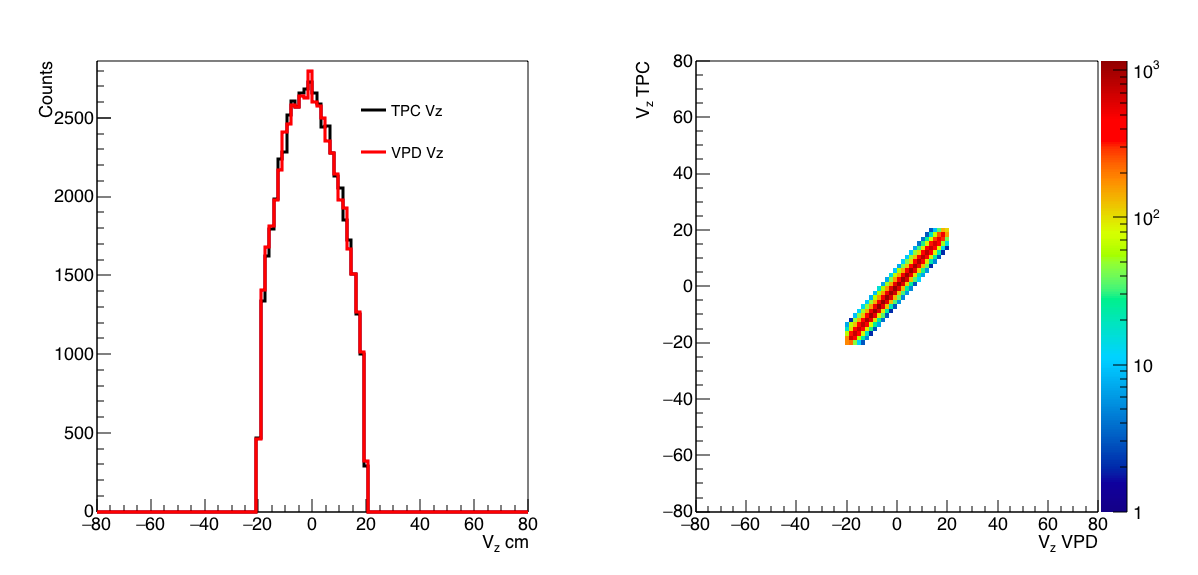
Figure 6: Vertex distributions after shifting Vz vpd, requiring that the tpc vz and vpd vz be within 6 cm of one another so that we know that that the tpc vertex is (mostly) in time and centered in STAR.

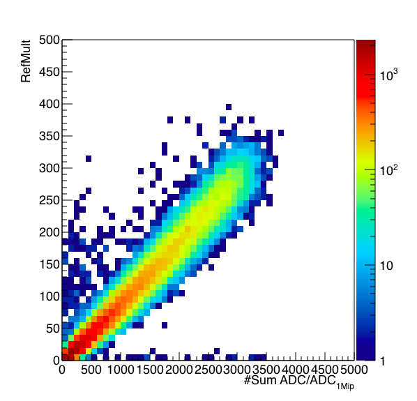
Figure 7: Refmult versus sum ADC EPD for our selected events.  We see that we've cleaned up a lot of the mess in Figure 2, there are still a few vertices that have more than the expected number of tracks in them.  One can spend a lot of time looking into this, but I won't at the moment.

For the slew corrections, I will perform the easiest automatic procedure.  For each tile I will take the profile from the distribution.  This value will then be subtracted from the TAC value in a given event if the tile had that particular value of nMIP.  I am choosing a bin size of 1 MIP, one could do this more finely but let's start with this.

The distributions can be seen at (sorry about the legends, but doesn't matter so much): drupal.star.bnl.gov/STAR/system/files/tacfit_04182018.pdf


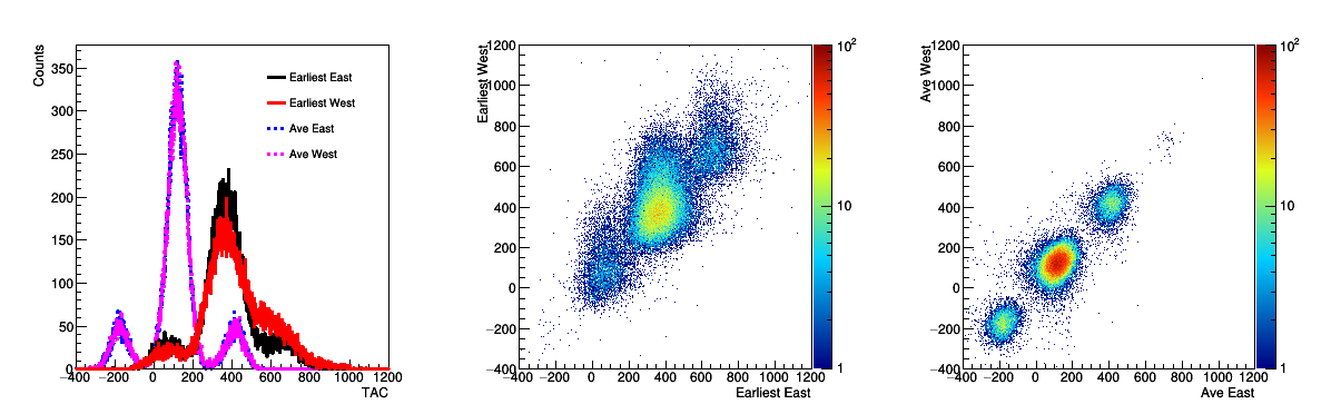
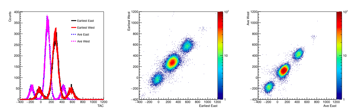
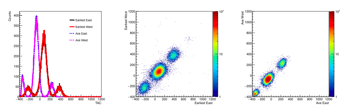
Figure 8: (Left) Fastest time East (black), west (red), average time east (blue), west (purple).  (Middle) Fastest time east vs fastest time west.  (Right) Average time East vs average time west.

In Figure 8 I started to include the average time rather than merely the fastest time.  The fastest time is what can be used in the trigger algorithm, but offline we can calculate the average time.  The fastest time will be dominated by the tails of the distributions, which is why it is shifted to higher TAC.  We also see that by switching to average time we can see the main bunch as well as the satellites more clearly, this also shows a tremendous improvement from the non-slew corrected data before.

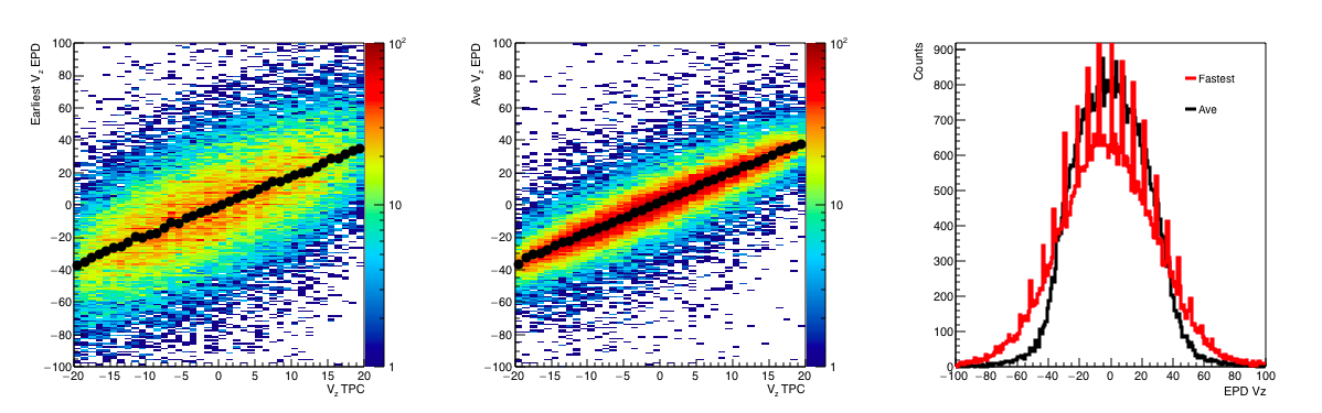
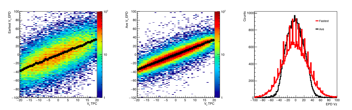
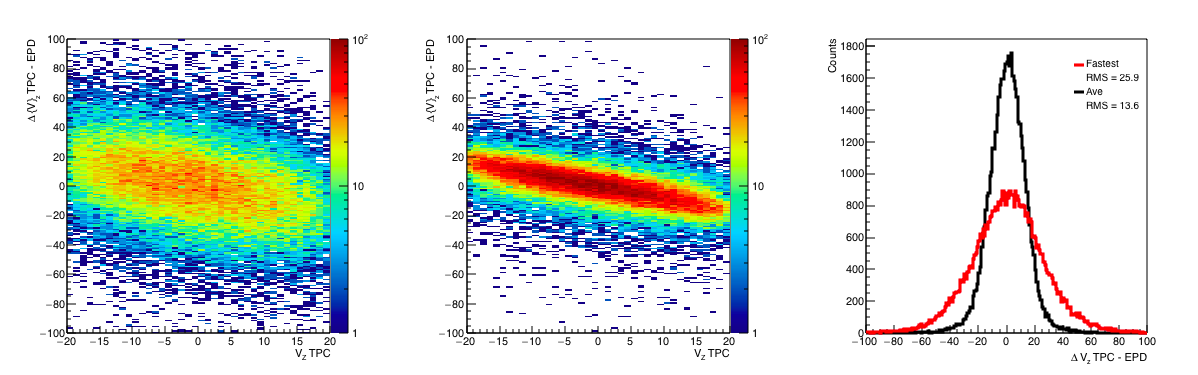
Figure 9: (Left) Fast EPD Vz vs Vz TPC Bz.  (Middle) Average EPD Vz vs TPC Vz. (Left) Projections of the L and M, showing the vertex distribution.  Fastest can still have this "beating" as we are subtracting 2 integers.

Figure 9 shows us the calculated EPD Vz (Delta TAC x 15.6 x 0.03 = Vz in cm).  The distribution for the average is much more tightly correlated so we see that the resolution is better, though  it does seem to have more of a slope to it than the fastest time distribution.

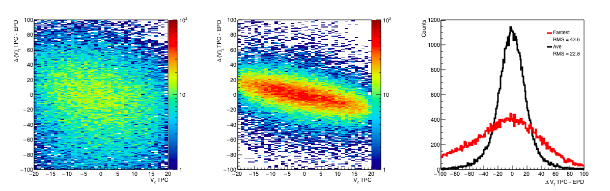
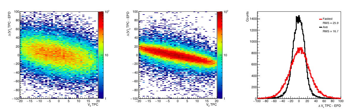
Figure 10: (Left) The difference in Vz between the TPC and the EPD for the fastest Vertex.  (Middle) The difference in Vz between the TPC and the EPD for the average TAC Vertex. (Right) Projections of L and M on the y-axis.  The width of this distribution is our spatial resolution.

In Figure 10 we see a first look of the resolution.  For the fastest TAC, we find a resolution of 43.6 cm (43.6 / 0.03 = 1.45 ns) and for the average TAC, we find a resolution of 22.8 (22.8/0.03 = 0.76 ns).  The average definitely improves our resolution.  However, looking at the resulting TAC vs ADC distributions: drupal.star.bnl.gov/STAR/system/files/tacfit_Corrv1_04192018.pdf I see there is room for improvement.  For one, the crude calibration method seems to be 200 ch too high (I think that the changing shape plus the effect of the satellites changes it.)  Another is that the change happens so rapidly that the 1 Mip values are all over the place.  Another is that it seems most of the real physics dies out at about 15 Mips.  

First I tried to add a -200 offset to the calibrated TAC, my worry was mainly that for the average calculation that the offset would come in many times over.  However, the results were absolutely the same, so let's forget this.

Next I will require the ADC correspond to 1 < ADC/1Mip ADC < 15, in order to maximize real signal and to stay away from the region where the rapid change in TAC vs ADC makes the slew correction difficult.

I will repeat the figures, all with the label Figure 11.

From this we see that excluding the badly corrected data and the landau fluctuations improves the timing resolution to: 0.56 ns.

I did some other fast looks, cutting on the corrected TAC to remove the outliers improves the resolution as well.  Increasing the nMip cut greater than 1 decreases the resolution.  I think we could probably improve things quite a bit by making a better slew correction for the low ADC signals.  Decreasing the upper cut doesn't really change things that much.  I also tried to recenter the total vertex distribution so that epd vz = 0 on average when tpc vz = 0, but this also did not really improve the resolution.  I did not want to adjust the slope as ideally we would only perform global operations to the EPD data and not based on an external factor.

The best case scenario here has:
Tac Corr = TAC - slew - 200
|Tac Corr| < 400
1 < nMip < 15

The plots (figure 12) from this are as follows:

From here, we see that our best resolution is 13.6, which corresponds to (13.6/0.03 = 0.45 ns).  One can then argue that using the RMS isn't quite right as this is influenced by the tails, so if we fit with a Gaussian, we find:

Figure 13: Final resolution plot for this study.  A spatial resolution of 11.8 cm corresponds to 0.39 ns.