In order to choose which 24 super-sectors are the best for the EPD, we need to have a way of quantifying what best means.  One could argue that best means all the tiles in a given SS perform well, there are some SS where this is true.  There are others where one tile has a signal that is reduced by half.  If we have to choose between some of these, what should be our method?

For using the EPD to determine the centrality of a collision, not all tiles are equally useful.  To determine this, I used some UrQMD trees given to me by Bill Llope for the energies of:
sqrt(s_NN) = 7.7, 11.5, 14.5, 19.6 GeV

I assumed that Vz = 0 in all cases.

I selected only protons, anti-protons, pi+ and pi- as particles able to leave a signal in the EPD.  I then used the StEpd code to project these particles to the Epd surface and determine which tile they hit.  I then keep track of the information versus tiles.

First, looking at the raw pseudorapidity for these particles:

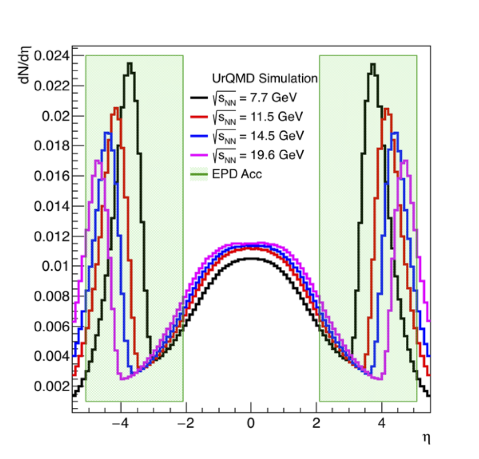
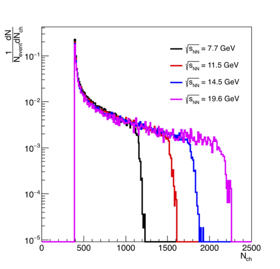
Figure 1: On the lef dN/deta versus eta for all 4 energies.  The EPD acceptance (for Vz = 0) is shown in green.  The beam rapidity sweeps through the EPD acceptance at these energies.  On the right is the total charged particle multiplicity for |eta| < 5.1.  This looks as expected.

We can then look at the charged multiplicity within the EPD itself:

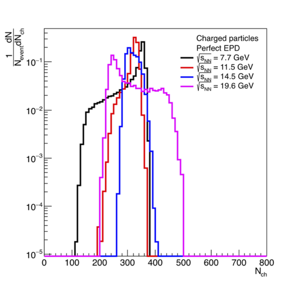
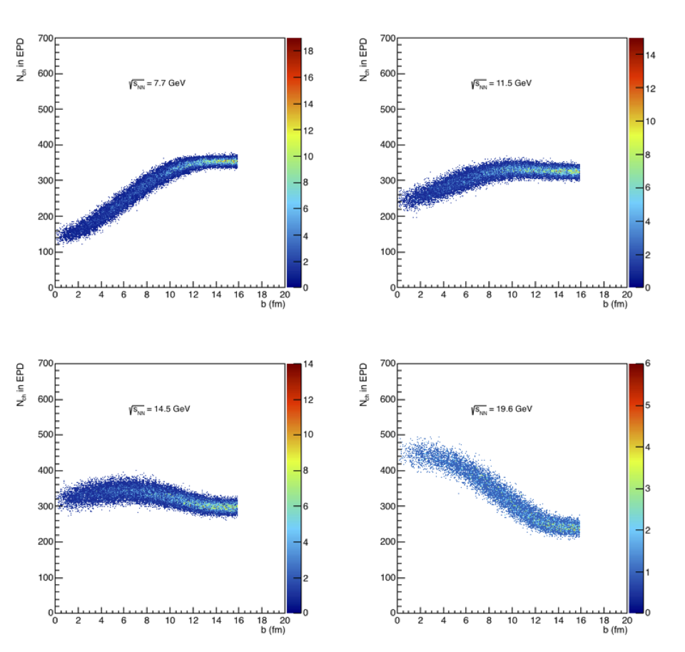
Figure 2: On the left is the charged particle multiplicity within the EPD acceptance.  The distribution switches from the distribution seen at higher energies to flip around at the lower energies, depending on whether the "mid-rapidity" or beam-remnant charged particle multiplicities dominate.  On the right is the distribution of the charged particle multiplicity in the EPD versus the impact parameter versus energy.   We see that in the lower right, the distribution is what we are more used to seeing with an increased in the number of particles for the most central events, whereas it is the reverse for 7.7.   What is potentially more difficult is the distribution is relatively flat for 11.5 and 14.5 GeV.

Since we know precisely what the impact parameter is of a given event, we can look at different bins in centrality:

Figure 3:  For all 4 energies the total charged particle multiplicity within the EPD is shown in black.  The charged particle distribution in the EPD for 4 centrality bins, chosen by the impact parameter b are shown in the various colors.  We see here that there is very little difference in 11.5 and 14.5 GeV.

The situation in figure 3 looks dire, unless one thinks about the fact that some etas should be very sensitive.  The issue will partially be that it is not clear how good a job UrQMD does at predicting the beam remnants, but it is what we have.  First looking at the average number of hits in each tile, versus the position of the supersector:

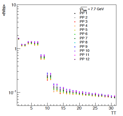
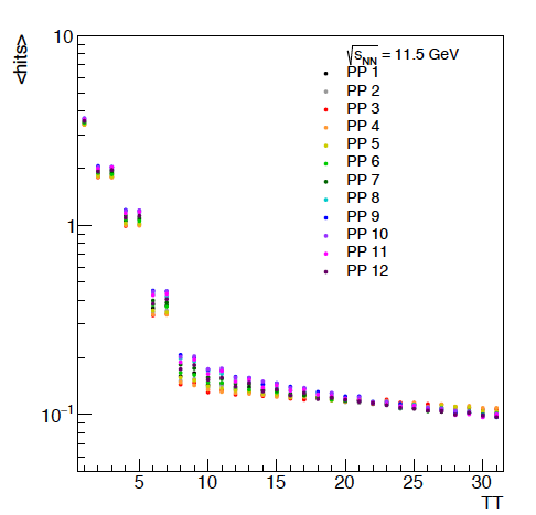
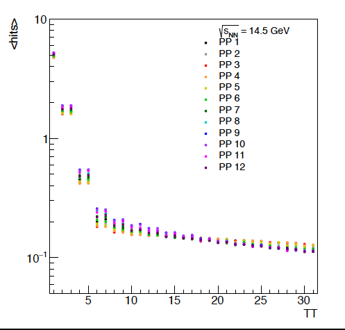
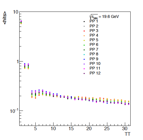
Figure 4: The average hits per tile versus energy.  It should be noted that there will be a discontinuity going from 1 to 2 as tile 1 spans twice the phi angle that any of the other tiles do.  Additionally, it is not surprising that the pairs of tiles perform similarly.  For the lowest energies, it looks like the first 5 or so rows of the EPD have the potential to be the most differential.  The offset in these different PP is due to flow, as the reaction plan is always oriented at phi = 0 in these events.  This will be useful when we study the event plane resolution.

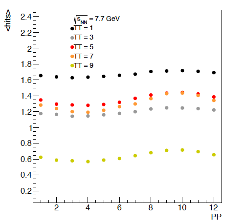
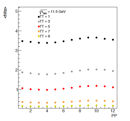
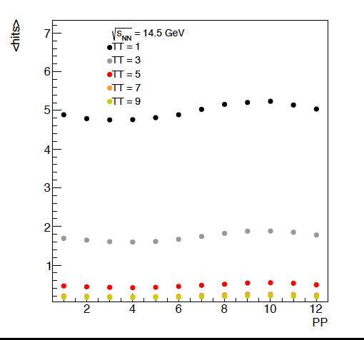
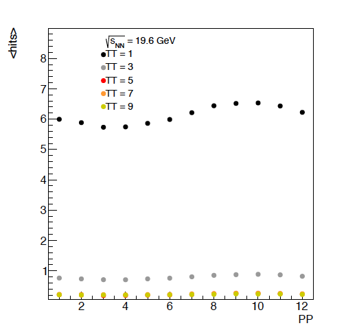
Figure 5:  The average hits versus super sector position (PP).  Given that the reaction plane is always at phi = 0, we can see the modulation here.  This is only for the first 5 rings in eta.

It is more fair to look at this distribution eta ring by eta ring as below.

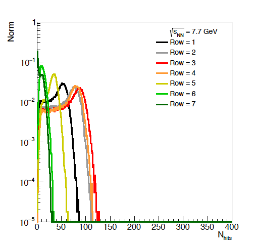
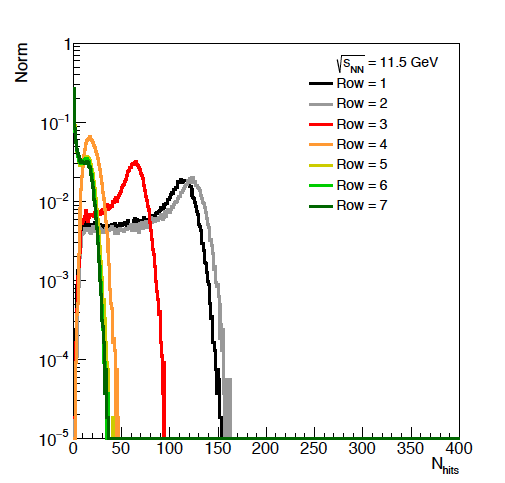
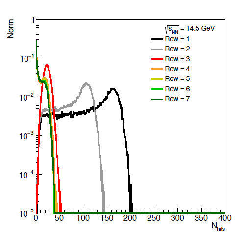
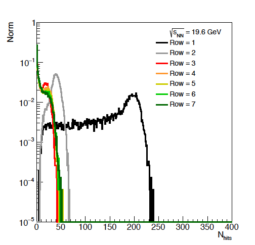
Figure 6: Average hits per eta ring versus energies. 

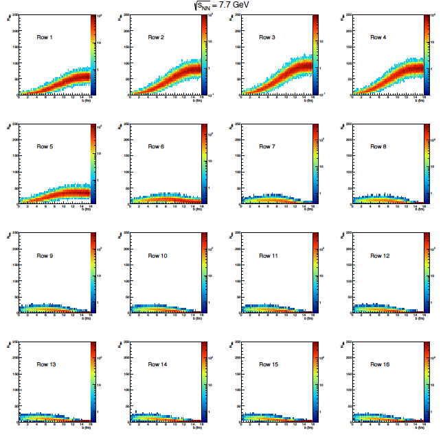
Figure 7: Nch in the EPD versus impact parameter in each eta ring for 7.7 GeV.

Figure 8: Nch in the EPD versus impact parameter in each eta ring for 11.5 GeV.

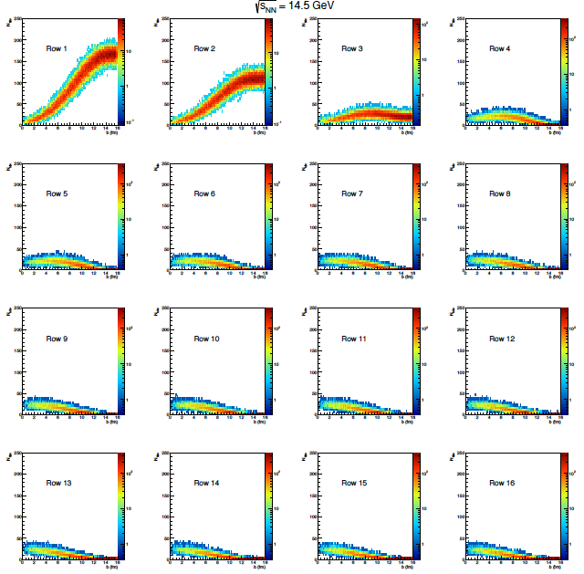
Figure 9: Nch in the EPD versus impact parameter in each eta ring for 14.5 GeV.

Figure 10: Nch in the EPD versus impact parameter in each eta ring for 19.6 GeV.

First I did a quick check to see what happened if I did some broad cuts, only considering the first ring group.  (Rows 1-3, tiles 1 -5).

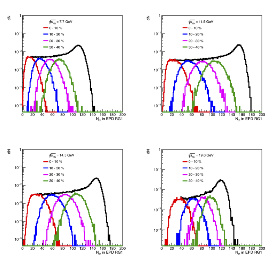
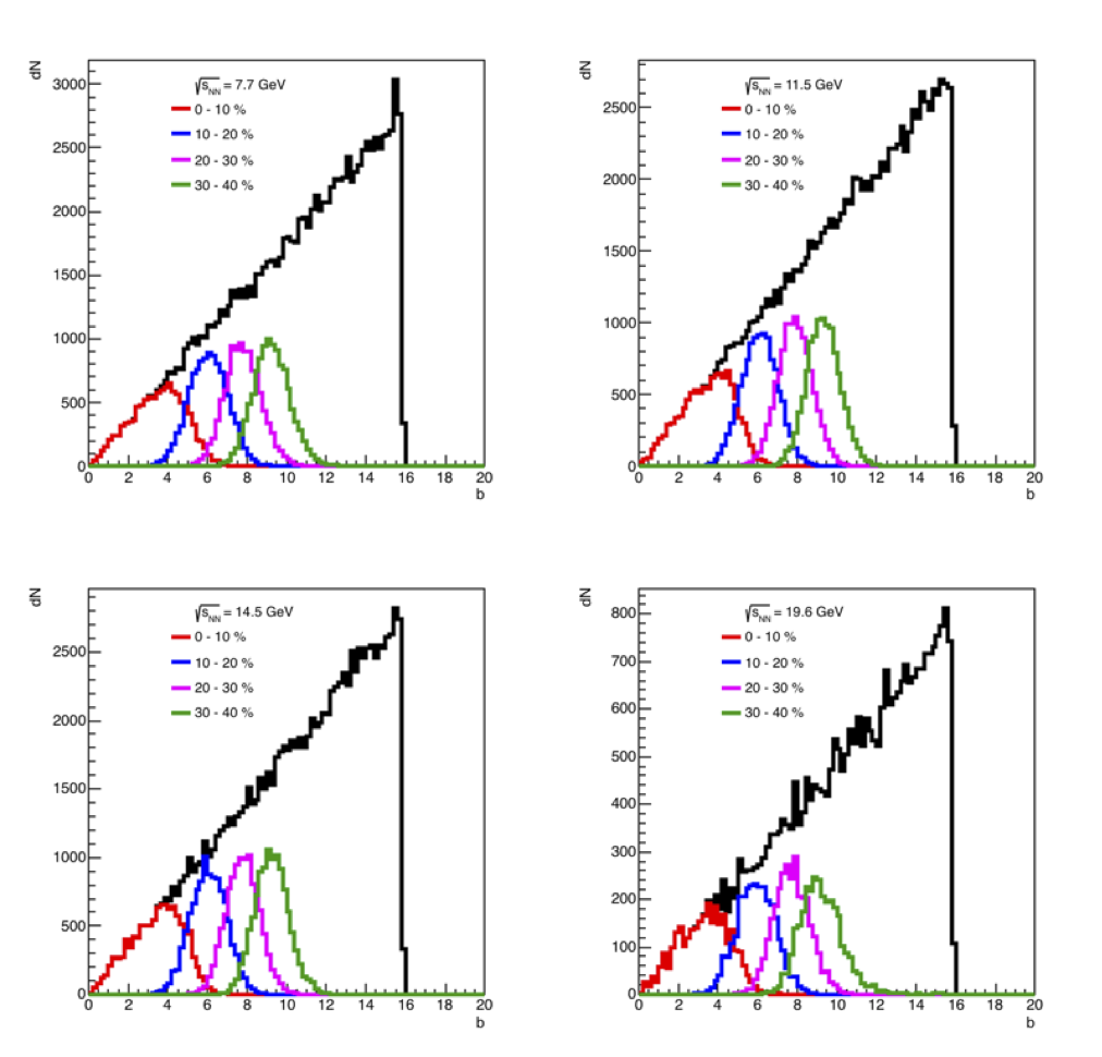
Figure 11: On the left is the distribution in a given ring group for all centralities.  The 4 centrality bins were chosen by selecting the impact parameter and then plotting the charged particles.  Note that even for 19.6 GeV, by looking at the high rapidity ring, the inverse relationship between centrality and number of charged particles in the EPD can be seen.  On the right, the distribution is shown in impact parameter, given a choice on Nch in the EPD.  This was chosen by assuming the efficiency was constant with respect to impact parameter (which is true in this simulation) and using the Nch_epd to determine the cut.

A couple of comments.... one is that depending on the beam fragments may be difficult, this should be discussed.  Of course, one can always do this in a data driven way once the BES data is available to us, but having the philosophy decided ahead of time would be useful.  This is especially important for deciding which 24 super sectors are the best.  The low numbered tiles seem most important in this case, unless we decide that we would prefer to rely on "mid-rapidity" production.  The problem there is the counts will be especially low....

So I started by seeing what happens if we only used the first row for centrality determination.  First, I "fit" each of the distributions, mainly to look to see when the average Nhits gets above the next integer value.  In the data, we will only have integer results, so I wanted to be able to determine an impact parameter for 2 hits, for 3, etc.

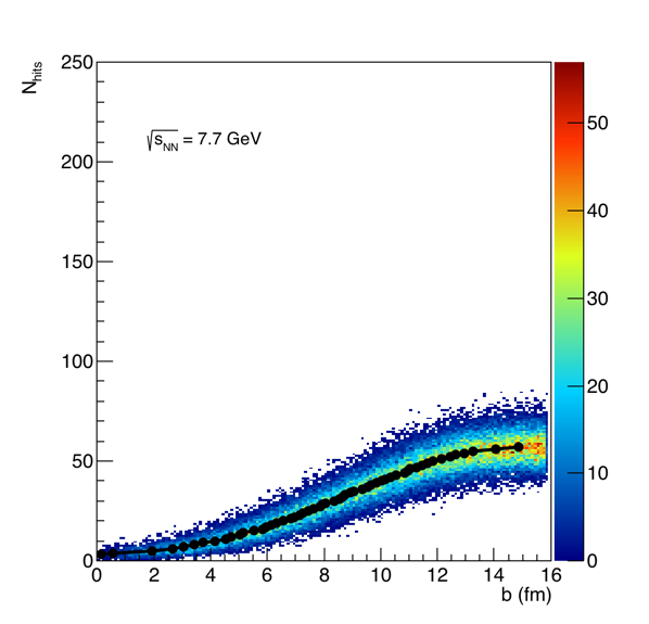
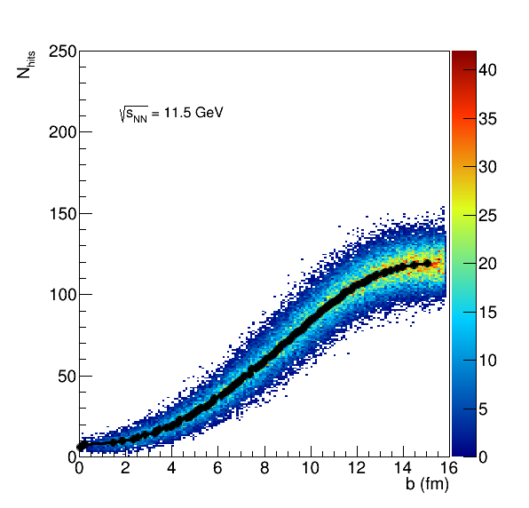
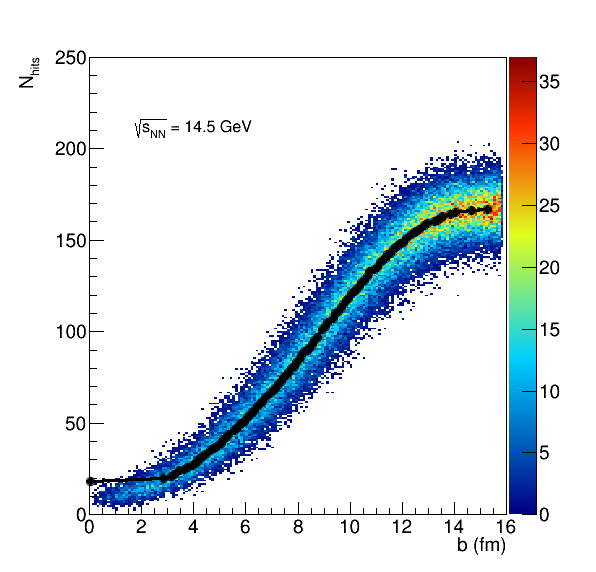
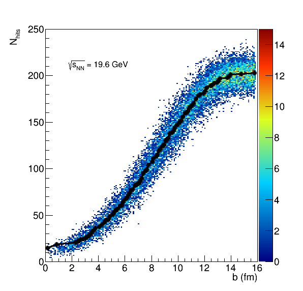
Figure 12: The fit to the b vs hits in the EPD, row 1 for the 4 different energies.

I then ran through the simulation again, for every event look at the difference between the "calculated" b and the real b.

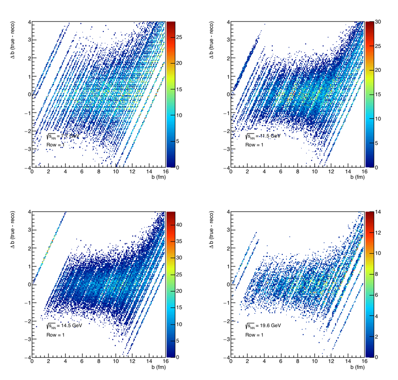
Figure 13: The difference between the calculated b and the actual b.  The stripes are due to the integer nature of the number of hits in the EPD.  The projection of these plots onto the Y axis gives us the resolution.

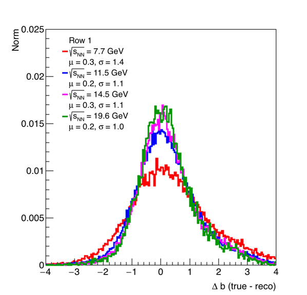
Figure 14: Resolution for only using row1 of the EPD for centrality determination.  This is the projection to the Y axis of the figures in 13, and then normalized by dividing by the total number of counts.