As a number of the items on my status page are intertwined, here is my plan.  As the steps are completed, I can add them to this blog or add links to new blogs, depending on how much stuff needs to be added.

The Few Day Plan

1. Focus only on the 303 runs with trigger levels "C" for the preliminary result. For the paper, or sooner if there is time, the extra 43 runs can be added.  The integrated luminoscity of the 43 runs left out (for now) is 11% of the integrated luminoscity of the combined 43+304 runs.
2. Look at the eta distribution in MC (for the pi0 signal) and in data, with Z vertex in +/- 120 (since this cut is in the MC filter) and no eta or detector eta cuts.  From these, an eta cut will be determined.
3. Within this eta cut, the data background template fit will be preformed, and plots of the mass distributions, chi^2/NDF, and number of pi0s will be considered, for each of the following Z-vertex cuts and detector eta cuts.  There are 6 (2x3) cases.  The Z-cuts are related to a previous study showing that this improved the comparison, though the study didn't include the trigger emulator for the Pythia sample.  It is hoped now that the MC is also cut on the trigger, the >-50 cut will no longer be relevant.  Studies by Dave U. suggest one contribution to the low mass shoulder is correlated with high detector radius, and thus the cuts on small detector eta.  Of the six cases, the one with the best data/MC comparision (without removing too many statistics) will be chosen
   • Z in [-120, 120] (cut A)
   • Z in [-50, 120] (cut B)
   • det. eta > 1.085, i.e. nominal value (cut 0)
   • det. eta > 1.1427, i.e. one tower (cut 1)
   • det. eta > 1.2023, i.e. two towers (cut 2)
4. Revist the eta cut (Step 2) within the new cuts of Step 3.
5. Add in beam crossing cut and reduce upper pT bin to smaller value (since no statistics in the upper part of the bin) and rerun full analysis scripts with the latest cuts.

This plan should cover all open issues with the exception of finalizing the documentation and the systematics.

Step 2: Eta distributions

Attached are the eta distributions for each pT bin--one pdf file for the Monte Carlo, which has been cut on "type a," the purist signal, and one pdf file for data, with eta vs mass per pT bin.  Thus while the MC is looking at the purest signal, the data includes pi0s and background.  It can be noted that the decision for the eta range is consitent for both samples.  The cut of 0.8 to 2.0 is chosen as the nominal value, which corresponds to the optimal setting for pi0s with pT in 8-10 GeV.

Step 3: Template Fits with various cuts

In contrast to the fit described in the blog from August 1st,  the histograms are not shifted by a bin width, but instead fit to functional forms with an energy scale factor.  The shapes that turn out to be the best are

• Signal: sum of two skewed Gaussians with common mean
• Conversion Background: single skewed Gaussian
• Other: cubic polynomial

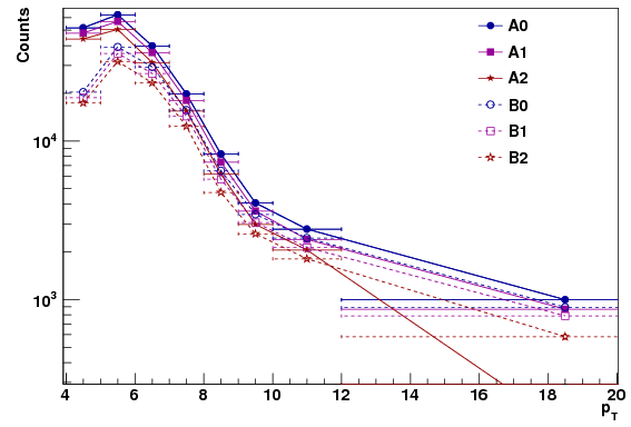
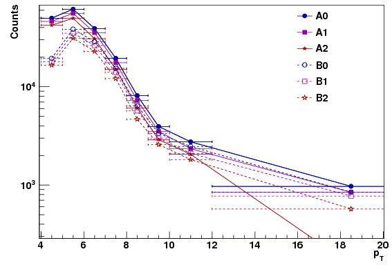
The fits of these templates are generally quite good (chi^2/ndf about 1).  Full details will be in forthcoming documentation.   Templates were made for each of the six (2x3) cuts listed above.  While all templates were fit to functions using the mass range 0.1 to 0.5 GeV, the data was fit to the templates in either 0.1 to 0.5 GeV or 0.11 to 0.5 GeV.  Attached are the plots showing the data, the functions, and the residual for all the fits.  Each pdf contains all the pT bins, and there are 2x3x2=12 pdf files (two Z cuts, 3 detector eta cuts, and two lower thresholds for the fit range).  The following plots show the chi^2/NDF for the fits as well as the number of estimated signal counts.  Uncertainties are not fully propagated.  Figure 1 is for lower fit range of 0.1 GeV, and second (right) panel is for the lower fit range of 0.11 GeV.

Figure 1: Starting at 0.1 GeV

Figure 2: Starting at 0.11 GeV

While  While both the detector eta and vertex Z cut do improve the chi^2/NDF, the estimated amount of counts drops and thus the reconstruction efficiency must also drop.  Note that the number of counts does not vary significantly with the shift of the lower value of the fit range.  The detector eta cut was intended to reduce some of the area where the data and Monte Carlo do not agree.  However, the fit range is designed to avoid most of the mass region where this occurs, so it was anticipated that the detector eta cut could have a minor effect (as it does).  The Z-cut also significantly reduces the chi^2/ndf.  By studying the residuals in the attached plots, one can see that the high chi^2/ndf in the lower pT bins is due to the pi0 peak being narrower in Monte Carlo than in data.  Most likely this is due to material missing in the simulation.  However, the improvement in chi^2/ndf does not seem worth the cost in statistics, and so the conclusion is to not use any vertex Z or detector eta cuts.

Step 4: Revist the Physics Eta Cut

No need, since it was decided not to introduce any of the cuts suggested in step 3.

Step 5: Tie up loose ends

In progress--the subject for another blog.

NOTE ABOUT ATTACHED PLOTS:

In the plots starting at 0.11, the yellow residual plot includes one too many bins on the low side, i.e. the first non-zero bin in the residual is the 0.105 to 0.11 GeV bin, which is actually not included in the fit.  This is just a mistake in the plot, but does not effect the computed chi^2 or any other values.