Investigation of BTOW scale using Jacobian peak "position"

Ideally the reconstructed Z mass would be used to set the BTOW scale for measurement of high ET electrons in the W analysis, however the yield in Run 9 is very small.  One possible alternative method of determining the absolute scale is to compare the measured Jacobian peak to the expected Jacobian peak (from simulation).  This analysis is similar to the method used at the Tevatron to fit the W mass from the electron pT and W transverse mass distributions, except here I'm assuming the simulation has the W mass right and determining the BTOW absolute scale.  Some details of the CDF and D0 analysis can be found in their recent W mass papers, where I stole this idea.  There is a nice description in the CDF paper in section II. D. 

Note: 1) All the plots shown on this page use Matt's calibration from electron E/p at 200 GeV

           2) All the plots below are for W+ as the W- statistics are not sufficient for a similar study.

 

Template Distributions:

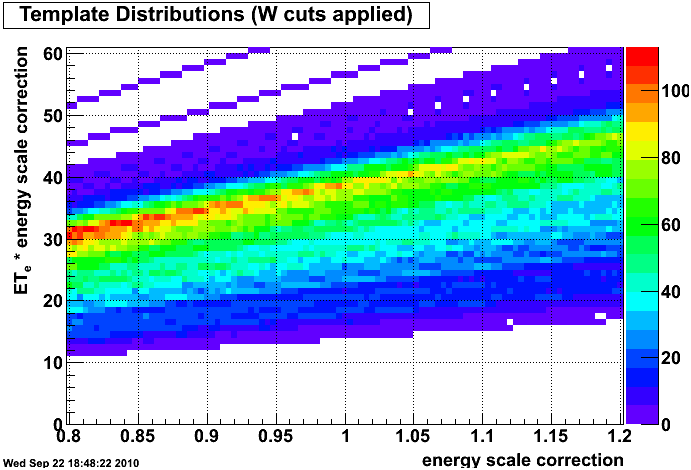
First I found template Jacobian Peak distributions from the simulation shifted by different energy scale factors [0.8,1.2].  The distributions are thrown electron ET for events that pass all our W cuts.  Below is a plot of the template distributions.

Figure 1: Thrown ET * energy scale factor  vs.  energy scale factor

 

 

Maximum likelihood fitting:

To compare the template Jacobian Peak distributions to the data I used the binned likelihood fitting procedure where the likelihood is defined as

where n_i is the measured yield and m_i is the expected yield in the i^th bin, and the goal is to minimize: - ln ( L ).  The uncertainty determined as the value of the scale factor where - ln ( L ) + ln ( L_max ) = 0.5  

All fits were done in the ET range of [30,50] GeV.

 

W MC simulated "data" proof of principle:

A first test of this method was to shift the gains up by 5% for the W MC sample and use the reconstructed MC electron ET distribution as simulated "data" to see if this method can determine the known gain shift from a reconstructed distribution.  The plot below shows the - ln ( L ) for the different possible energy scale factors.

Figure 2: - ln ( Likelihood ) (left),  chi^2 (center), and reco/thrown E (right): for the different possible energy scale factors (simulated data gains scaled by 1.05)

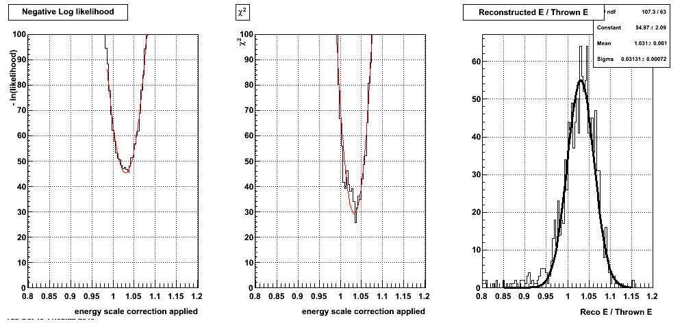
The energy scale factor with the maximum likelihood in figure 2 is 1.032 +/- 0.005, and the chi^2 = 11.92 for 10 DOF for this scale factor.  The reconstructed/thrown energy has a mean of 1.031 +/- 0.001 shown on the right.  So the gain shift matches the reconstructed/thrown energy as expected. 

 

Another test of this method was to shift the gains down by 5% for the W MC sample and use the reconstructed MC electron ET distribution as simulated "data" to see if this method can determine the known gain shift from a reconstructed distribution.  The plot below shows the - ln ( L ) for the different possible energy scale factors.

Figure 3: - ln ( Likelihood ) (left),  chi^2 (center), and reco/thrown E (right): for the different possible energy scale factors (simulated data gains scaled by 0.95)

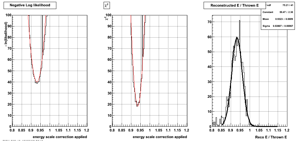
The energy scale factor with the maximum likelihood in figure 3 is 0.931 +/- 0.005, and the chi^2 = 18.07 for 10 DOF for this scale factor.  The reconstructed/thrown energy has a mean of 0.932 +/- 0.001 shown on the right.  So the gain shift matches the reconstructed/thrown energy as expected.

 

So it appears possible to determine a gain shift (in either direction) from the simulated "data" with this method.

 

Data:

The same method was applied to the background subtracted electron ET distribution from the data.  A range of additional smearings were applied to the templates and a resolution of 7% had the best fit to the data so it is applied to the template fit distributions used here.

Figure 4: - ln ( Likelihood ) (left) and chi^2 (right) for different possible energy scale factors

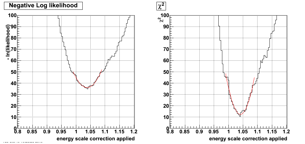
Figure 5:  Background subtracted data (black) and normalized template distribution with energy scale of 1.038 applied (red)

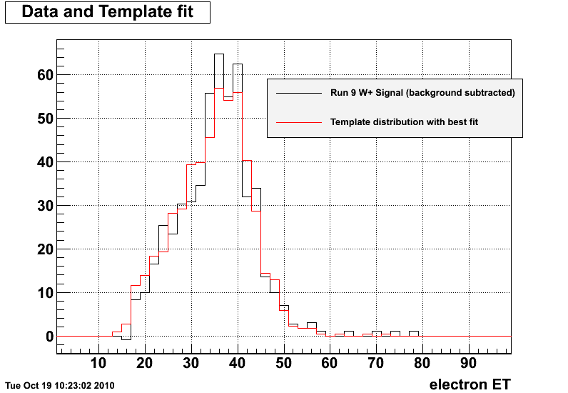
The energy scale factor with the maximum likelihood for the BTOW gain correction is 1.038 +/- 0.010, and the chi^2 = 12.49 for 10 DOF for this scale factor.    Figure 5 shows the data distribution and the template distribution with the determined energy scale applied.

 

Systematic Uncertainty Checks:

1) Fit Range: 

    a) Hold upper bound on fit (ET = 50 GeV) and vary lower bound

lower bound of fit (GeV)	24	26	28
btow scale factor	1.036	1.039	1.039
uncertainty	0.009	0.009	0.009

    b) Hold lower bount on fit (ET = 30 GeV) and vary upper bound

upper bound of fit (GeV)	52	54	56
btow scale factor	1.038	1.038	1.042
uncertainty	0.009	0.009	0.009

    So varying the upper and lower bounds of the fit range has a small effect on the extracted BTOW gain correction.

2) Smearing applied to template distributions:

    A range of smearing was applied to the template distributions from 0% - 10%.  The largest scale factor obtained with the different smearings was 1.056, and the smallest was 1.034.  So the choice of additional smearing applied to the template fits has an effect on the extracted BTOW gain correction, which is non-negligible.

3) RHICBOS vs PYTHIA : does the jacobian peak "shape" bias the extracted BTOW gain correction?

Figure 6: Thrown PYTHIA positron ET (black) and RHICBOS positron ET (green)

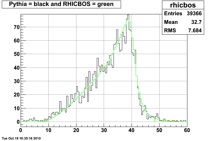
The above distributions were used to weight the PYTHIA events contribution to the template distributions so the templates now reflect what RHICBOS predicts for the Jacobian peak "shape".  Then the entire fitting procedure is done again and the result is figure 7 below.

Figure 7: - ln ( Likelihood ) (left) and chi^2 (right) for RHICBOS weighting of input ET distribution

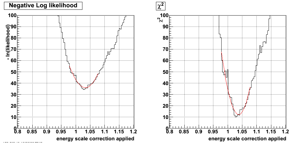
The scale factor obtained with the Rhicbos weighting is 1.033 +/- 0.009.   So for the RHICBOS Jacobian peak shape doesn't differ drastically from the PYTHIA shape, and thus the template fits are relatively unaffected.

4) Varying background model (ie. using different shapes for "data-driven" background to extract scale correction)

The systematic uncertainty in the background model is found by varying the shape of the "data-driven" background distribution by varying the signed pt balance cut used to define the background sample as well as varying the normalization range for scaling the background shape to the data.  Figure 8 shows the different signal distribution with all the possible choices of background shape and normalization.  Clearly in the fitted region (ET=[30,50] GeV), this will have a minimal impact on the correction factor calculated.

Figure 8:  Background subtracted W signal with nominal background shape (black) and all other possible shapes and normalization ranges (red).

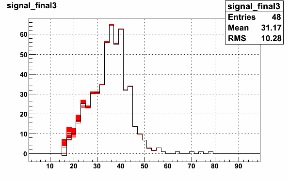
The largest scale factor obtained with the different background shapes and normalizations was 1.039, and the smallest was 1.037.

5) Eta Dependence

As a check of the eta dependence of the BTOW scale correction I divided the data into 2 bins in detector eta (|eta| < 0.5 and 0.5 < |eta| < 1.0).  To use the same method as above I used the same background procedure as before, but now separating the background in the 2 eta bins to give background subtracted spectra for each eta bin to be compared to template fits that are divided into the 2 eta bins.  Below are some plots of the - ln ( Likelihood ) distributions and data/template fit overlayed as in Figure 4 and 5 above which is summed over all |eta|

Figure 9:  - ln ( Likelihood ) for different possible energy scale factors on the left and  background subtracted data (black) and templage fit (red) on the right  |eta| < 0.5

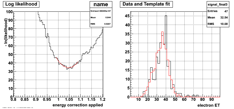
The energy scale factor with the maximum likelihood for the BTOW gain correction for |eta| < 0.5 is 1.047 +/- 0.012  .

Figure 10:  - ln ( Likelihood ) for different possible energy scale factors on the left and  background subtracted data (black) and templage fit (red) on the right  0.5 < |eta| < 1.0

The energy scale factor with the maximum likelihood for the BTOW gain correction for 0.5 < |eta| < 1.0 is 1.043 +/- 0.018.

So the BTOW gain corrections found in the 2 |eta| bins are consistent with what was found when averaging over all |eta|.

6) Other statistical tests (Kolmogorov–Smirnov test, others?)

    Still to do.

 

Summary of systematic uncertainties

Systematic	Uncertainty Calculated
Fit range	0.4%
Smearing applied to template distributions	1.8%
Jacobian "shape" (RHICBOS vs PYTHIA)	0.5%
Varying background model	0.1%
Eta Dependence	0.9%
E/p analysis of low E electrons (ie. Matt's gains)	1.9%

 

The first 5 uncertaities above are combined linearly ("perfectly correlated") to be conservative and sum to 3.7%.  Combining this quadratically with the uncertainty determined by Matt from the E/p analysis (1.9% mainly due to field flip) and the statistical uncertainty of the likelihood method (1%) gives a total uncertainty on the BTOW scale of 4.3%.

 

Z Mass consistency check:  Similar to the above method using the likelihood fits to the Jacobian peak to determine the BTOW scale correction, a measurement of the Z mass can be used as well.  Below is a figure of the reconstructed Z mass with the same gains used as in the analysis above for the likelihood fits.

Figure 11: Z mass from all Run 9 data

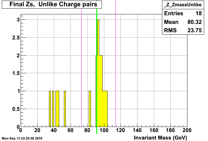
Including all the points between the pink lines the mean measured Z mass = 94.69 GeV, which is 3.8% larger than the PDG value. 

If the possible outlier at 83 is excluded the mean measured Z mass = 95.67 GeV, which is 4.9% larger than the PDG value.

So the BTOW scale correction one finds from the Z mass measurement is consistent with what was found using the maximum likelihood method described above.