Here is a progress report on estimating run-by-run led variations. www.star.bnl.gov/protected/spin/yuxip/report_6.5.pdf

It also contains the conclusion of bXIng offset value for the 59 fills (fill15200 - fill15419) that cover all of our data.

the complete set of plots relevant to the above report can be found here:

1. mean ADC of LED events for 19 cells connected to LED channel 1 (21 runs of day 80): www.star.bnl.gov/protected/spin/yuxip/CelladcLED_080_1_21_1.pdf

2.distribution of "diff", as defined in the report, over 200 runs: www.star.bnl.gov/protected/spin/yuxip/CellRunDep_1_200.pdf

3. projected mean LED adc v.s. measured, for 6 runs on day 95 based on run12080001: www.star.bnl.gov/protected/spin/yuxip/CellproLED_1_095_6.pdf

Further explanation on the above progress report

I added colors to some of the terms in the formulae below, in order for them to be self-explanatory, but they did not show up as colorful terms on drupal. So I am attaching a pdf file with the same context as the following. www.star.bnl.gov/protected/spin/yuxip/further%20explanation.pdf

1. In order to describe the variation of LED intensity, I tried to the extract the common mode of mean ADC variation, on a run-by-run basis.

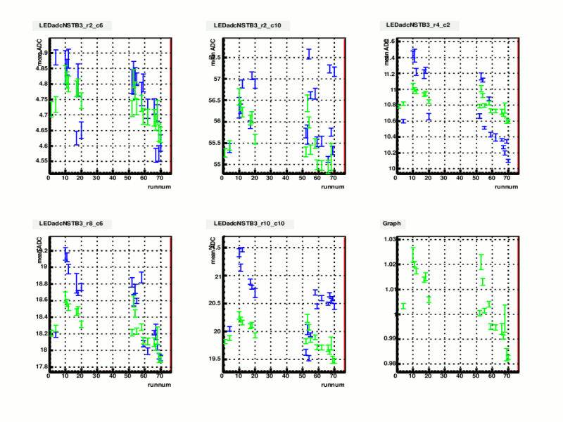
                        Figure 1. an example of finding the percentage variation, data from 21 runs on day 80

The first 5 frames of figure 1 are 5 out of the 19 cells which are connected to the same LED pulser. X axis is the reduced run number ( run number - 12080000 ) , y axis is the average ADC over the run.

Blue points are the actual mean ADC, measured for each run ( from run 12080001 to 12080070)

Green points are deduced from the 6th frame, which represents the percentage variation of the mean ADC for this group of 19 cells, scaled to the 1st point ( run12080001, as run(1), baserun).

                In the last frame, Green point ( run(i) ) = ADC( run (i) ) / ADC ( run (1) ), averaged over these 19 cells.

Whereas for the first 5 frames, the green points of the last frame was rescaled to the mean ADC of the base run for each cell. Take Cell(k) for example,

               In the kth frame, Green point( run(m), cell(k) ) = Green point( run(m) ) of the last frame * ADC( run(1), cell(k) ) .

The basic assumption was that averaged percentage variation (relative to the baserun) would represent the change of LED intensity over these runs. So those green points in the first 5 frames are the estimate of mean ADC for each run, if the gain remains to be the same as that of the baserun.

I am calculating the ratio ADC( run (i) ) / ADC ( run (1) ) because the intensity of LED pulses might not be equally shared among those cells. But this ratio is independent of the absolute intensity that was delivered to the cell. So when calculating the mean of ADC variation, cells with low ADC counts would be treated equally as those with higher ADC counts. As an simple example, if we measure the mean ADC of 2 cells, for 2 runs.

                                        run1(adc)      run2(adc)            var.

                     Cell 1:         1                        2                    100%

                     Cell 2:        100                   150                 50%

                        sum:        101                   152                 50.5%     -->biased to the cell with higher ADC counts

                     But the current method will give (100% + 50%)  / 2 = 75% . Essentially I am computing the average of variation, instead of the variation of average

This brings up another issure, that cells with very unstable gains will likely mess up the correspondence between the average of ADC variation and the change of pulser intensity

So when calculating the green point, we only want to include stable cells. This will benefit from the recent work of Chris

2. To check the validity of the above assumption, and to see if the green points are good estimate of LED intensity variation. I turned to examine the distribution of the difference between green and blue dots for each cell, over 200 runs from day 80 to day 95.

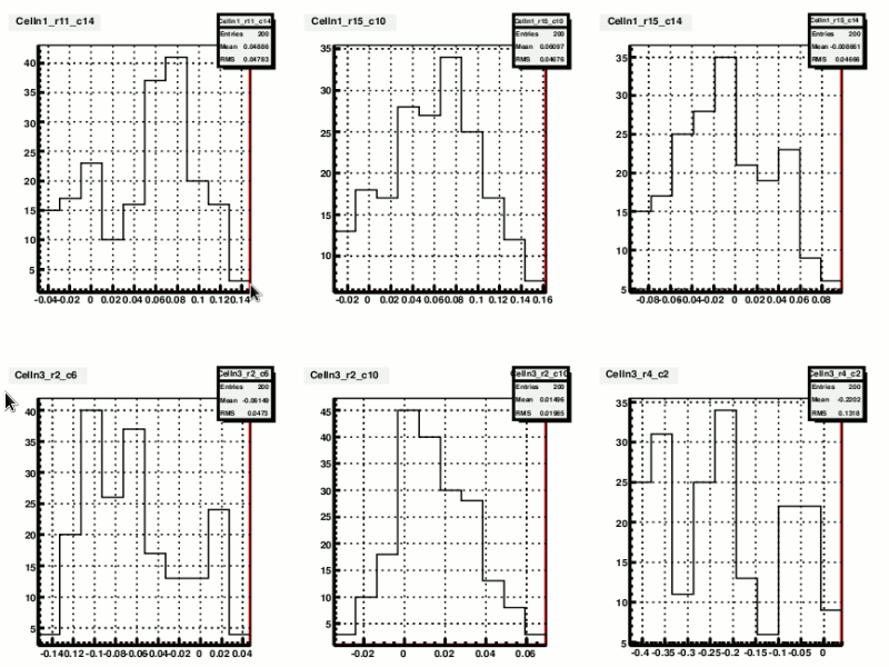
    For each cell, a variable "diff" is defined as diff( run(j) ) = ADC( run(j) ) / ADC( run(j),estimated ) - 1, simply the ratio of blue over green point, then minus 1. Below is the distribution of diff for several cells from the same group.

                                  Figure 2. Distribution of "diff" variable

      Before I can draw any conclusion from these distributions  It should be pointed out that we can make fairly resonable arguments concerning the distinction between tube gain variations v.s LED intensity variation. Without manually tweaking the HV settings, the fluctuations of actual gain are more of a random nature, typically with higher frequency compared to the variation of pulser intensity, which depends on room temperature etc. So we can think of the observed ADC variations as being composed of a fast gain fluctuation (Gaussian), plus a slow drift of the mean of this gaussian distribution.

     If the behavior of pulser intensity is very well described, we could have a handle on the above slow componet of those ADC variations. In this case, it can be shown that "diff" as defined above is equal to the variation of tube gain relative to the gain at the time of baserun.

               diff( run(j) ) =  ADC( run(j) ) / ADC( run(j),estimated ) - 1 = [ gain( run(j) ) - gain( run(1) ) ] / gain( run(1) )

and the "diff" variable for a specific cell would have a Gaussian distribution centered around 0, since the drift of the mean of this Gaussian distribution at different runs had been  cancelled. On the contrary, if the estimated ADC (green points) failed to describe the intensity variation, this "diff" variable would be ended up having mutiple Gaussian components with different mean values, like the last frame of figure 2. One example of this failure is in the case of including one or more unstable cells into to the estimation of averaged variation ( green dots of the last frame in figure 1.)

3. Apply the same method to a different dataset consisting of runs from different days.

      these are run12080001, as the base run similar to the above scenario under item 1, and 6 runs from day 95.

                       Figure 3. measured ADC v.s estimated ADC, as a function of run number

    Here I calculated the averaged variation in the same way as I did to find the green dots in the last frame of figure 1. Then I rescaled those green dots to the measured ADC of the baserun for each cell, to get the blue points in figure 3. So these blue points are the same as the green points in the first 5 frames of figure 1, they represent what the mean ADC would be if the tube gain is a constant and equals to the gain at the time of baserun. The pink point are the actual measured mean ADC over the run. And for each frame, the first pink point is the mean ADC of base run (run12080001).

    If the blue points are close to pink points, it means the observed variation of mean ADC( relative to the baserun ) can be well accounted for by the change of LED pulser intensity, therefore the actual gain of the tube did not change much, compared to that of the baserun.Take the 6th frame of figure 3 for example  In the previous time dependent gain correction scheme, the 10% drop in mean ADC would result in a 10% increase in the tube gain (ADC*gain = Energy). But in the current method, since the observed the mean ADC is very close to the predicted one, when taking into account of the pulser intensity variation, the predicted tube gain would be very close to the gain of base run.

  In practice, the new method can be incorporated into the current time dependent correction routine by introducing a run dependent (or time dependent) nominal LED ADC. This nominal LED adc used to be set to the mean ADC of the base run, which corresponds to the gain correction factors calibrated for the base run. But here the nominal LED adc needs to be reset to the predicted mean ADC for each run (blue points of figure 3), in order to account for the pulser intensity variations.