Since I had a pretty good shower fit for photons that enter the detector with almost zero incident angle ( see previous post ), the next step would be to incorporate non-zero incident angle effect into the shower function. Because we have seen that the evolution of the actual shower shape as a function of pseudorapidity was the domiant factor that obscures the reconstructed photon position. In the mean time, the fitting procedure developed for previous symmetric shower function is also helpful to fold in the incident angle effect due the specific method that we chose to address the problem.

Basically, when incident angle is involved the shower shape that we see at the transverse detector plane is actually a projection of the 3D shower distribution, with z-component mixed in to the transverse profile. Therefore the most exactly way to describe this kind of shower shape would be to have a differential 2D shower function T(x,y,z), convoluted with the longitudinal shower development G(z), so that the final shower function will be something like:

                                                                                                 (1)

But in reality, we dont know the form of the differential shower function T(x,y). It represents the transverse shower profile within an infinitesimal longitudinal z-slice. So the best thing we can do is to approximate the above integral by a finite sum:

                                                                                                  (2)

 , where we split up the total shower distribution into several z-slices with finite thickness, and measure the transver shower profile of each slice (T hat). Then all the z-slices are added up with an weighting factor g_i which approximates the longitudinal shower development. Incident angle effect comes into the equation througth dependence of the shower center (x_c, y_c) of each slice on z coordinate:

                                                                                                                                   (3)

In the above equation (x_cmax, yc_max) are the position of the shower center for the z-slice with the highestt weight, this coordinate will be reported as the position of the photon. In summary, (x_cmax,yc_max, tan(thetaX) tan(thetaY)) are the variable parameters that we will get from the fit. They can be initialized by the simliar parameters from the clustering.

At this point, it becomes clear that the pieces we need from simulation are those g_i's and T_hat's in e.q.(2). I divided up the vertical shower shape from the same group of cells used in my previous analysis (blue group) into 6 slices. For each slice, I only collect the optical photons which were generated within that slice and arrived at the photon cathode. The shower fit for each slice are shown below.

                                                                zbin_1,   0 ~ 7.5cm                                                                                                              zbin_2 ,   7.5 ~ 15cm

                                                                    zbin_3,   15~22.5cm                                                                                                             zbin_4,   22.5~ 30cm                                                           

                                                             zbin_5,   30 ~ 37.5cm                                                                                                                      zbin_6,  37.5 ~ 45cm

                                                                                                                        figure.1 shower fit in each z-slice

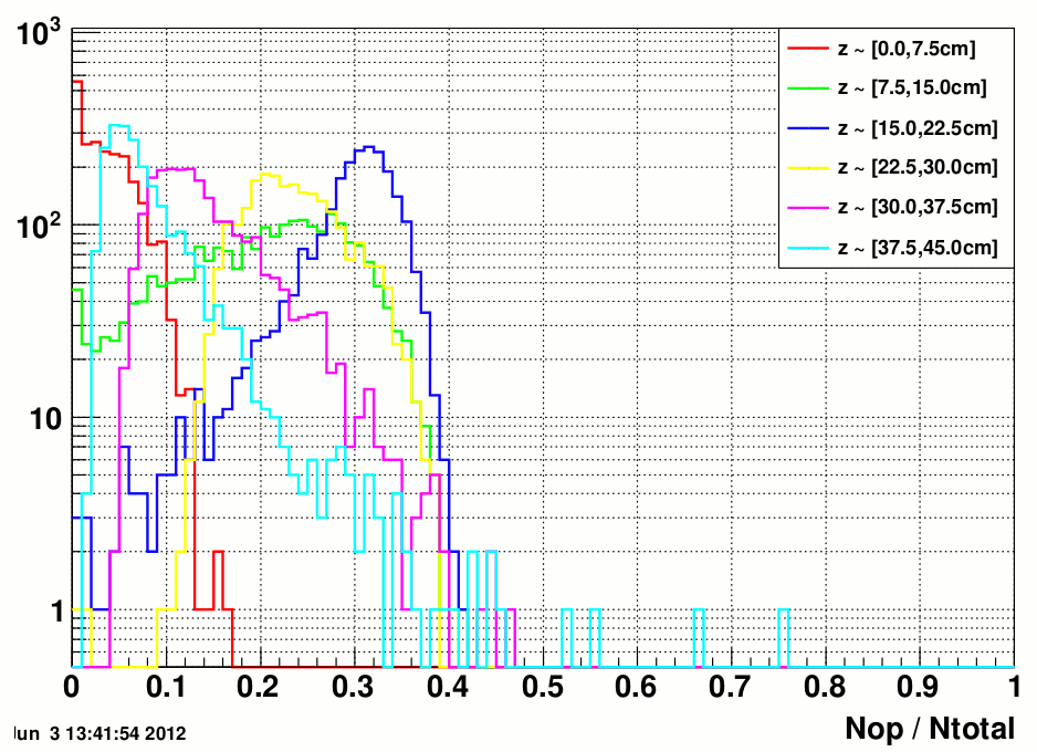
Each of these shower shapes is normalized within the same z-bin, namely frac. = # optical photons(x,y=0) / total # of optical photons in the same slice. From fit I get a set of parameters that describe T_hat in equation (2). The weighting factors are calculated by the ratio between # of optical photons from a specific z-slice to the total # of optical photons in the detector, as shown in figure 2.

                                                                                                 figure 2. # of optical photons generated in each z-slice, as a fraction of the total

The mean of each distribution is used as the weight of each shower function. As it can be seen the 3rd slice has the highest weight, therefore the shower center of the 3rd slice will be used as the (x_cmax, y_cmax) and reported as the reconstructed position of the photon. Combining all the pieces into e.q. (2), I fit the horizontal shower shape from the same group of 3x3 cells (figure.1 in previous post)

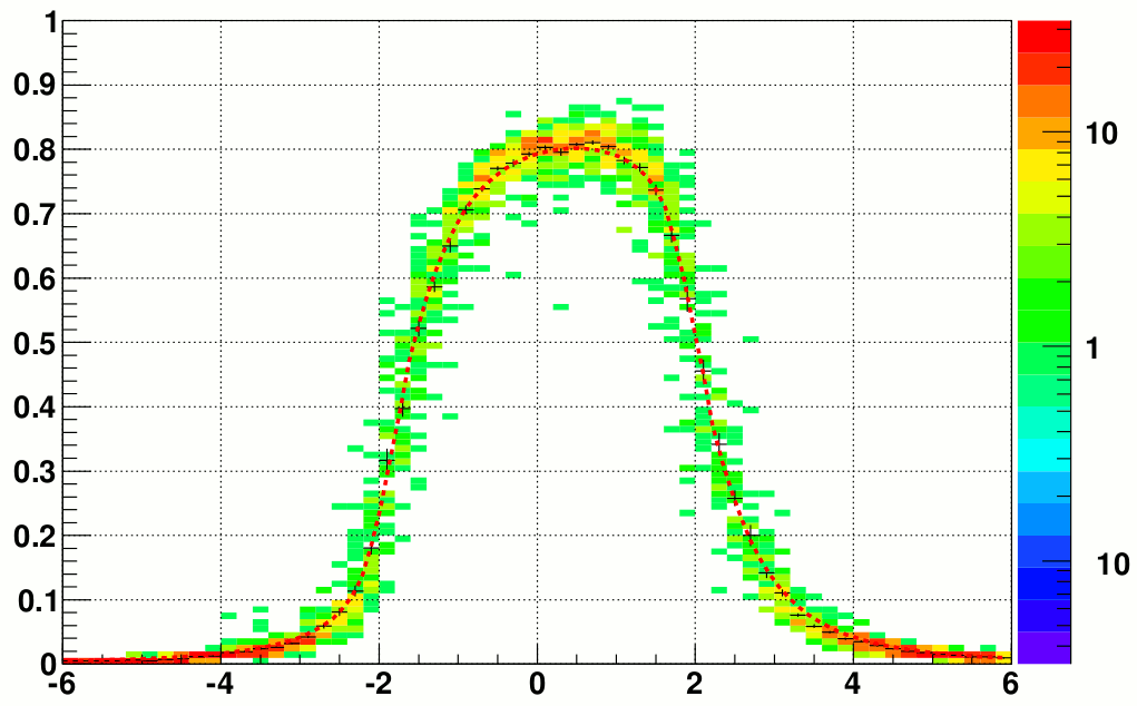
                                                                                                                                             figure.3 asymmetric shower fit

Notice that in simulation the shower shape was originally centered at the true position of the photon (x_0,y_0), calculated at the nominal shower max (z_max =  729.7cm). But x_cmax from the fit is equal to 0.26cm. That's because this position is evaluated at z = 735.45cm which is the depth of the 3rd z-slice. And we already know that the shower max of 40GeV photon is behind the nominal shower max.

The next step is to see if the skewness of the shower shape at small cell (row3,col3) could explain the fact that our data shower shape is wider than that in simulation (with zero incident angle). And to look at large cells particularly since the incident angle problem is more severe in there. And finally incorporate the asymmetric shower fit to the photon reconstruction routine.