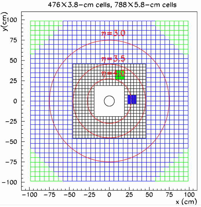
In the previous update I analyzed the simulated shower shape by looking at a group of 9 cells around nstb4_row3_col3( figure.1 in green). This area is located at north part of the small cell detector, next to the vertical axis (y). It turns out that the shower shape showed a visible skewness both in the x and y directions, therefore prevented me from getting a resonable fit with a symmetric shower function in order to set the baseline for studying the variation of the shower shapes when incident angle is involved.

As I got more statistics, I also turned to looked at a different region of the detector. This region is centered at nstb3/4_row11_col7 ( figure.1 in blue), almost lying on x-axis. Therefore the skewness along y direction is minimized. Actually only the 3 cells in central column (col7) are involved when I am looking at the vertical shower shapes. The requrements on selected clusters are:  1. the central cell row11_col7 must be the highest tower. 2. The x coordinate of true photon position must be within 1/5 of the cell width relative to the center of cell row11_col7. The second cut removed a lot of outliers in the shower center which appear to have very low energy fraction, due to their offset in x direction

                                                                                     Figure .1  3x3 cells group used for shower shape study

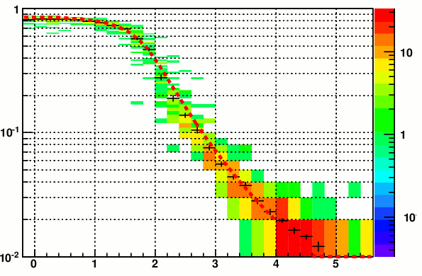
Then I fit the vertical shower shape by TMinuit, as shown in figure 2. The starting point of the fit is the default shower shape (top fraction ~ 85%)

                                                                                             Figure 2. fitted shower shape in simulation

    and the 6 parameters are:

a[1] = 1.06841, a[2] = 0.150087, a[3] = -0.171292, b[1] = 0.37491, b[2] = 0.860969, b[3]= 0.386676. There is no limit on any of the parameters during the fit. Notice that the sum of all a's is not exactly 1, which means these parameters need to be rescaled in defining the new shower function.

compared with the default parameters:

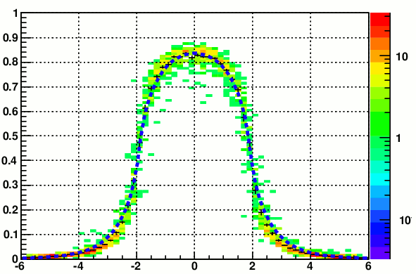
a[1] = 1.070804, a[2] = 0.167773, a[3] = -0.238578, b[1] = 0.535845, b[2] = 0.850233, b[3] = 2.382637. The largest difference is in b[3]. When I put some relatively loose constraints on these parameters I can have a better match on b[3], but I dont see any visible change in the actual shape. Figure 3. shows the default shower function on top of the same simulated shape.

                                                                                                    Figure 3. default shower function

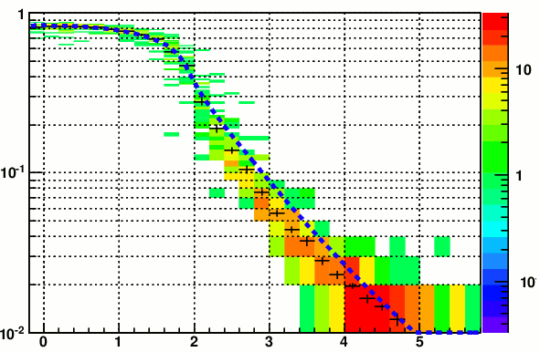
Figure 4 shows a comparison with Saroj's shower function which is believed to be a better estimate of the actual shower shape in data. But it turns out that this shape is wider than the simulation.

                                                                                                                        Figure 4. Saroj's shower function.

From figure 2. and 3. I think the conclusion is that the default shower function I used in the simulation pretty well describes the shower shape at zero incident angle. This is also supported by figure 1 and 3 a). in my previous post, where the deviation of reconstruced position from true position is the smallest at near 0 incident angle. All the other discrepancies come from the evolution of the shower shape as a function of the incident angle.

Now that I have a working procedure of fitting shower shapes, I begin to study the tranverse shower profile at different depth in the detector, and by overlapping multiple shower shapes from different depth with different offsets in their centroid it is possible to describe the skewed shower shape at finite incident angle. Technically I have found a way to record the Cherenkov photons generated at a specific depth in the lead glass. In this way I can look at shower shapes at different z-slices.

Link to figure 2, a)

Link to figure 2, b)

Link to figure 3, a)

Link to figure 3, b)

Link to figure 4, a)

Link to figure 4, b)