I've processed 14 fills of run11 data and have gone through the procedures of calculating background substracted asymmetries. Although I still have
problems in matching simulation with data especially at low energies, I decided to proceed with signal + background fits which allow for variable shapes.

In order to make contact with the preliminary result I use the same x_F binning: 40~60 GeV, 60~80 GeV and 80~100 GeV

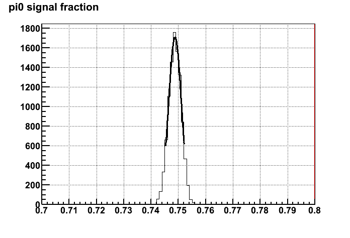
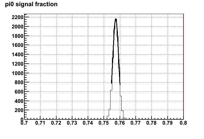
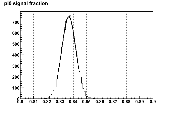
pi0 signal and backgrounds fits to the mass spectra

pi0 signal was fit to a skew Gaussian while background was 3rd order polynomial. The intial parameters of the shapes were derived from MC but
these parameters are not fixed in the fitting. I am currently only looking at JP2 triggered events.

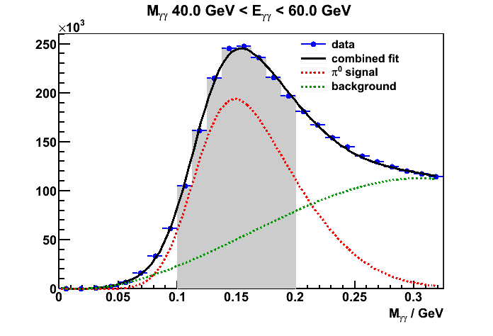
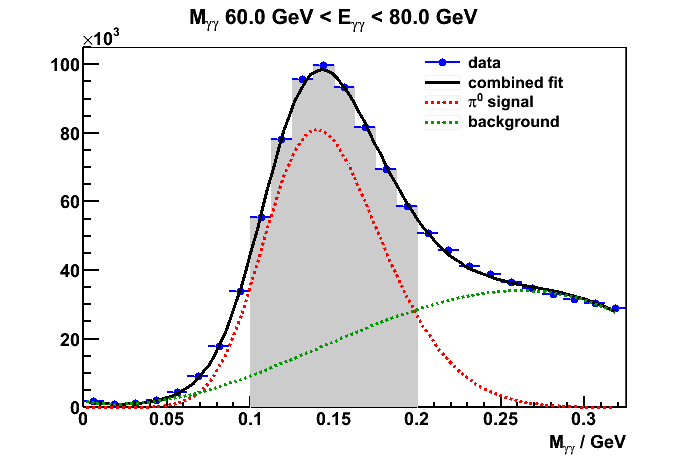
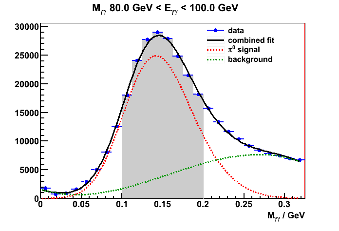
             Figure 1. signal + bkg fits to the diphoton mass spectra

I've selected a fixed mass window [0.1, 0.2] GeV to define the signal(peak) region.

signal fractions in the peak region

The integral of signal and background fits as a fraction of the combined fit in the peak region defines the signal and background fractions.
Figure 2 shows the signal fractions for the 3 energies bins.

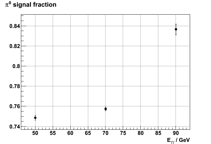
                                    Figure 2. pi0 signal fractions vs energy

The uncertainties of the signal fraction was calculated by running a toy MC instead of propagating the errors analytically
(which also assumes linear approximation). The goal of this toy MC is basically to see to what extent the calculated signal fraction
varies given the uncertainties of the signal + background fit. The procedure of this toy MC is as follows,

      1). From the fit I obtained the 8 parameters and their covariance matrix. Assuming these 8 parameters follow 8-dimensional Gaussian
            distribution with the same covariance matrix, then the problem reduces to the case where I can sample this 8-d Gaussian and calculate
            the corresponding signal fraction. The width of the distribution of the sampled signal fractions then defines its uncertainty.

      2). In practice it's very easy to generate 8 independent random variables that follow the same Gaussian/Normal distribution. In order to
            introduce a desired correlation among these variables one has to apply the Cholesky transformation(http://en.wikipedia.org/wiki/Cholesky_decomposition).
            Basically this transformation matrix was calculated by decomposing the target cov. matrix into a product of lower triangle matrix and its own transpose
           
            Cov = UU^T
           
            Then the U matrix can be used to transform those 8 independently normally distributed random variables into ones which correlate just as cov.

      3). So now after the Cholesky transformation I can calculated the corresponding signal fractions. I've sampled 10k replicas and plotted the distributions of signal
            fractions as shown in Figure 3. The covariance matrix of the transformed variables are indeed very close to the orignal covariance matrix from the fit.

                                       a). 40~60 GeV                                                                                                                                       b) 60~80 GeV

                                                 c). 80~100 GeV

             Figure 3. distribution of signal fractions with 10k replicas

raw asymmetries vs mass and background asymmetries

Figure 4 shows the raw asymmetries (w/o pol. correction) vs diphoton mass, using both the cross ratio method and cos_phi fitting.

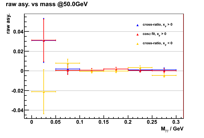
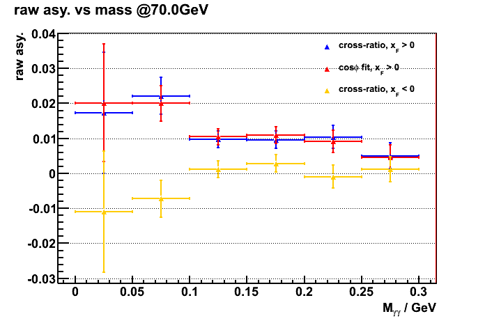
                                                    a). 40~60 GeV                                                                                                                                       b). 60~80 GeV

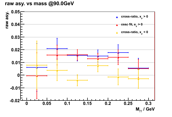
                                                 c). 80~100 GeV
                  Figure 4) raw asy. vs mass (no bkg subtraction)

Here the cross ratio method was implemented by dividing the phi space into 10 bins, and the phi dependent analyzing power A_N(phi) was calculating for
each pair of phi slice which are opposite to each other. Finally A_N(phi) for the 5 pairs are plotted vs cos(phi) (phi is the angle between the photon pair and x-axis)
from which the extracted slope is the single spin asymmetry A_N. Figure 5 a).shows an example of the cross ratio method I used here.

      
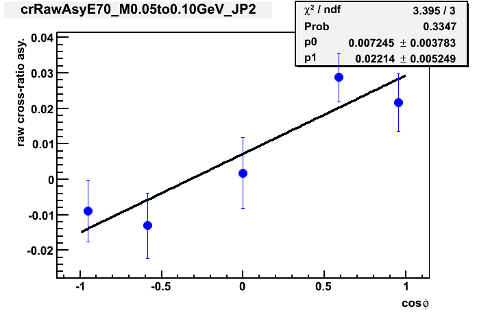
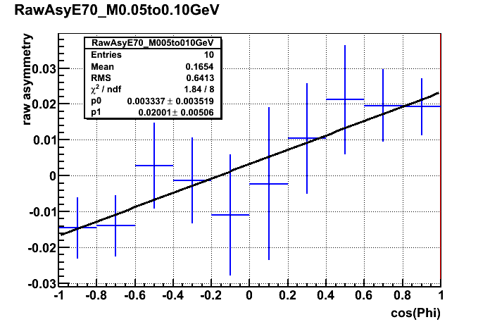
            Figure 5 a). cross ratio vs cos_phi for E = 70 GeV and 0.05 < M < 0.10 GeV                             Figure 5 b) raw yield asy. vs cos_phi for E = 70 GeV and 0.05 < M < 0.10 GeV

Whereas in the cos_phi fitting method, the raw asymmetries in pi0 yield (N_up - N_down)/(N_up + N_down) was plotted vs cos_phi. And the slope of the linear
fitting gives spin asymmetry A_N (before pol. correction) and the intercept gives luminosity ratio, as shown in Figure 5 b).

Since both method give very similar results I'll just show the cross ratio results from here on.

background subtracted asymmetries

From Figure 4 I calculated the total A_N (w/o background subtraction) for the signal region 0.1 ~ 0.2 GeV by taking the average of the corresponding 2 bins. And the background
asymmetry was calculated by taking the average of the remaining 4 bins on the side-band (0~0.1 GeV and 0.2 ~ 0.3 GeV). Signal fraction and its error are taken from Figure 3).
According to the following formula,

                                              
                              
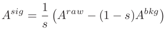
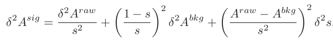
I calculated background subtracted A_N and its error, as shown in Figure 6, for both x_F > 0 and x_F < 0

         
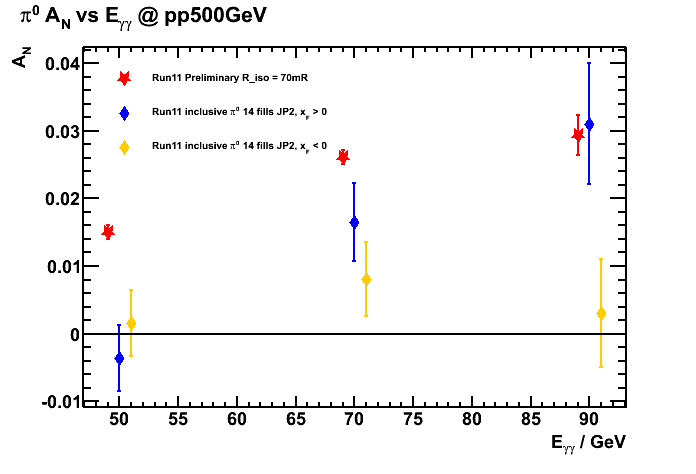
                          Figure 6. A_N vs energy. Red: Run11 preliminary results with isolated pi0. Blue: inclusivs pi0 A_N with ~half of  Run11
                                           statistics (with JP2 trigger) for x_F > 0. Yellow: inclusivs pi0 A_N for x_F < 0