We have been able to map out and run most of the frist step(smd slope fitting) of the EEMC calibration. In this step we have identified three sub steps:

1. First iteration of Runs:

This step is preformed by calling the script submit.pl and passing it two arguments, what run you want to get the histograms for and then what iteration number you are on. For the first argument you can give it a run number, for example: 10136009, or the command "all" to submit a job to the STAR servers to give you histogram files of the smd, pre/post, and tower for all the runs. A list of all the runs used is attached to this post in the form of an Excel spreadsheet.

Next the script bigSectloop.sh is called with one argument, the iteration number. This script will find all the histogram files and add them into summed histogram files for each sector/plane. For most of the following data that is presented all the runs are used. Discussed later are some findings when the runs are divided up into six groups that have close start run times. To all the smd summed histograms a fit is done to the slope to find the relative gain for each strip. These fits are then exported in the form of .pdf files that have the fits on the histograms for each section/plane, and .dat files that have the gain and gain error for each strip in a section/plane. Attached at the end are .zip files that have these files in them. Below are two histograms from these files:

Section 01 plane U strip number 001.

Section 08 plane V strip number 001.

 In order to see how the gains change in a section based on strip number a plot of strip gain versus strip number was done. In all graphs it can be seen that strips with higher strip number have larger error bars on them. All of these graphs are attached in a .zip file.

The gains from this fit where also compared to 2006 data to see how they have shifted over the years. The two below grahps are gain ratio plots. On the y-axis is the gain of 2009 over the gain of 2006. On the x-axis is the strip number. In these graphs any strip that had a zero gain or zero error from either 2009 or 2006 had its value set to -0.5. This was done so we could see and ID those strips in the plot.These plots are also attached in a .zip file.

2. Creating Bad Strip Mask:

With all of the gains now in data files, we need to generate a mask file that will remove all bad strips for the next step. Before this summer there was no code that created this mask file, so it was constructed and compared to the results of Jan's mask file from the 2006 calibration (Both of these masks are attached). This code looks into the .dat files for the run and will flag a strip with one of three reasons for being bad. The first is "Not Fibered", all of those that where listed as not fibered in Jan's list where also found in this new mask. The second is "No Signal, Dead Channel". If a strip has no counts in it and does not show up as not fibered it has stopped working and therefore is flagged here. Finally, "Too Few Counts". If a strip has less then 90 counts in the slope fitting area it will be flagged. This threshold was found by using Jan's previous mask list as a guide. Looking at his data it was found that the lowest number of counts that would be allow was about 90. This number was then used in this code to remove all of the strips with too few counts.

This mask file was checked against the histogram files and was found to ID the strips correctly. It was found, however, that a visual inspection was needed of the histograms to find any stuck bits or other oddities in the fits. These have also been added to the mask file and a reason for the flag.

3. Second Iteration of Runs:

After a mask file has been made, it and the .dat gain files produced by the fits are added to the code when the runs are submited to STAR. The resulting histogram files will now have all bad strips removed. This step then ends the first part of the overall EEMC calibration. We believe that the next step after this is use UxV coincidence alonge with the pre and post showers to ID mip signals that pass through all the layers.

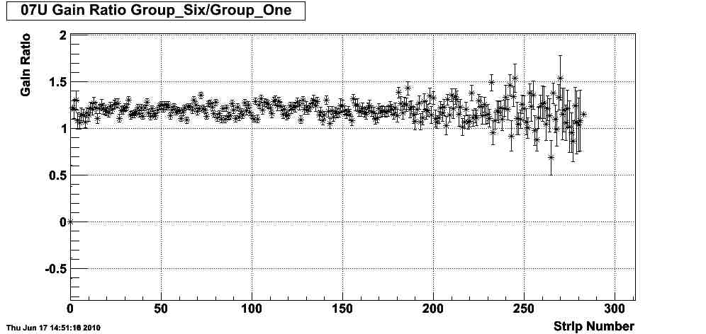
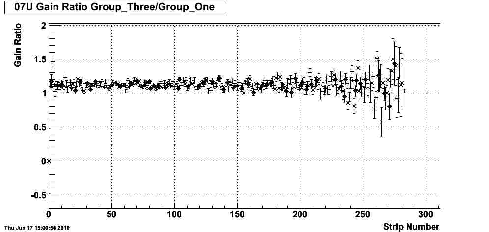
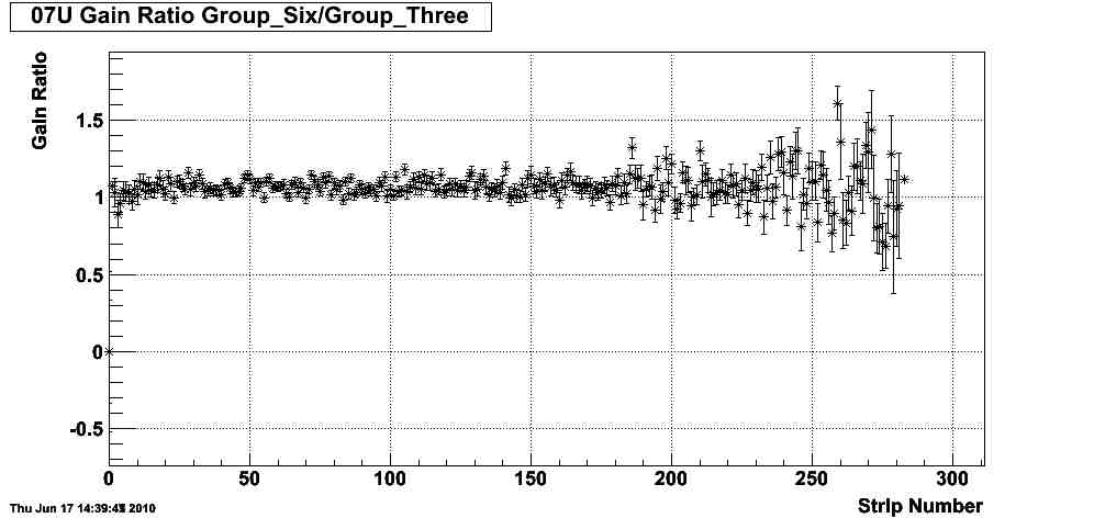
Interesting Observations with Grouped Runs:

The above analysis was done with all the runs summed together. We also divided the runs into six groups each containing about 23 runs each 10-12 days in length. These groups are noted in the runs.xls file. This grouping was done to see how much the gains shifted over the course of a few days. When comparing group six with the first, it was found that all the gains had sifted up by about 20%. Comparing group three with group six found a much smaller change in the gains. When group three was compared to group one a large shift was found again. This suggests that the large gain shift happened early on in the 2009 run. The below plots show this behavior. The ratio used is the gain of one group over another. The ratio shows that if the gain does not change between the two groups it will be one. As the gain of the group in the numerator increased the ratio will be greater then one.

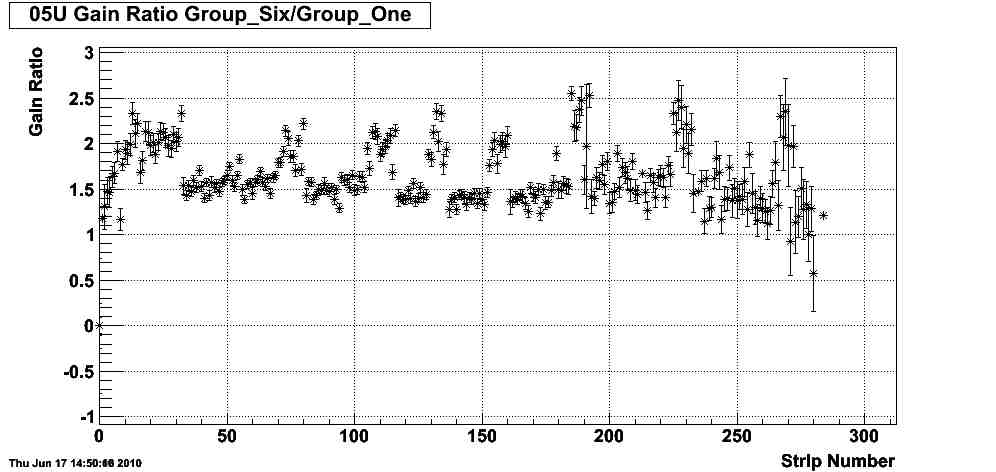
Greater Time Dependent Changes for sections 5, 8, and 12:

These observations also suggest that the gain changes over the course of the whole run. Sections 05U, 08U, 12U show the same but with added features. At current the reason for these jumps are not known. What is known is that when group six and group three are compared the jumps all but go away.These Observations are still very early, but the reason as to why this is happening is being looked into as the work continues.

Additional Information:

Attached to this post:

runs.xls  - Has all the runs used in calibration. Also has the runs set up into groups
smdAllMaskDay89v1.txt  - Jan's Mask file from 2006
smdMaskFile2010.txt  - 2009 Mask file made using code and visual inspection
allRunsDAT.zip  - All the .dat files for all smd sections, contains the gain information
allRunsPDF.zip  - All the .pdf files created that contain histograms and fits of the smd
gainPlots.zip  - All the gain plots for 2009 as .jpg files
gainRatioPlots.zip  - All the gain ratio plots between 2009 and 2006 as .jpg files

Location of files out at STAR:
/star/institutions/valpo/nramm/EEMC_cal/

     The EEMC_cal/ folder has a folder for all the runs and then each group of runs. It also has the gain plots for the changes in the gain between groups

Blog Post:

http://drupal.star.bnl.gov/STAR/blog/znault/2010/jun/15/creating-mask-file
http://drupal.star.bnl.gov/STAR/blog/znault/2010/jun/14/smd-iteration-results
http://drupal.star.bnl.gov/STAR/blog/znault/2010/jun/08/first-iteration-results
http://drupal.star.bnl.gov/STAR/blog/znault/2010/jun/04/running-scripts

http://drupal.star.bnl.gov/STAR/blog/nramm/2010/jun/17/grouped-run-datacharts-eemc-calibration