2008

Year 2008 posts

01 Jan

January 2008 posts

2008.01.30 Selecting gamma-jet candidates out of the jet trees

Ilya Selyuzhenkov January 30, 2008

Data set

jet trees by Murad Sarsour for pp2006 run, runId=7136022 (~60K events, no triggerId cuts yet)

Jets gross features

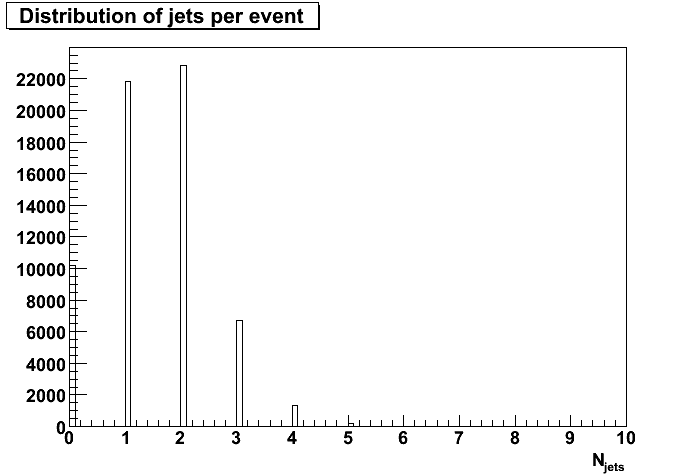
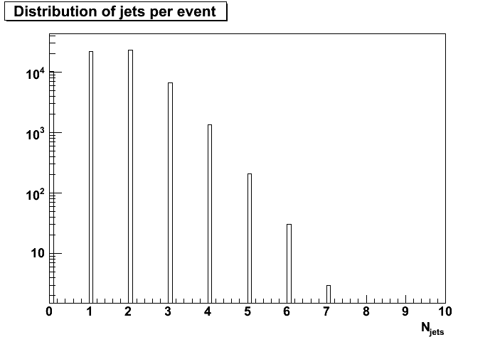
Figure 1: Distribution of number of jets per event. Same data on a log scale is here.
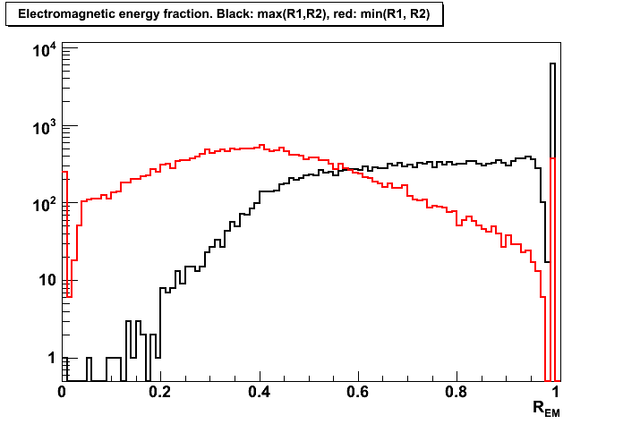
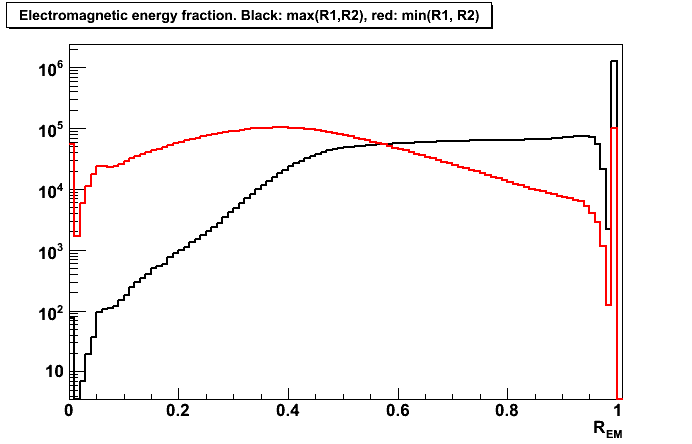
Figure 2: Distribution of electromagnetic energy (EM) fraction, R_EM, for di-jet events (number of jets/event = 2).
R_EM = [E_t(endcap)+E_t(barrel)]/E_t(total).
Black histogram is for R_EM1 = max(Ra, Rb), red is for R_EM2 = min(Ra, Rb).
Ra and Rb are EM fraction for jets in the di-jet event.
Same data on a log scale is here.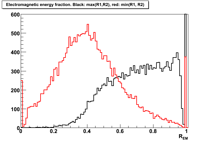

Gamma-jet isolation cuts list:

selecting di-jet events with one of the jet dominated by EM energy,
and another one with more hadronic energy:
R_EM1 >0.9 and R_EM2 < 0.9
selecting di-jet events with jets pointing opposite in azimuth:
cos(phi1 - phi2) < -0.9
requiring the number of associated charged tracks with a first jet (with maximum EM fraction) to be less than 2:
nChargeTracks1 < 2
requiring the number of fired EEMC towers associated with a first jet (with maximum EM fraction) to be 1 or 2:
0 < nEEMCtowers1 < 3

Applying gamma-jet isolation cuts

Figure 3: Distribution of eta vs number of EEMC towers for the first jet (with maximum EM fraction).
Cuts:1-3 applied (no 0 < nEEMCtowers1 < 3 cut).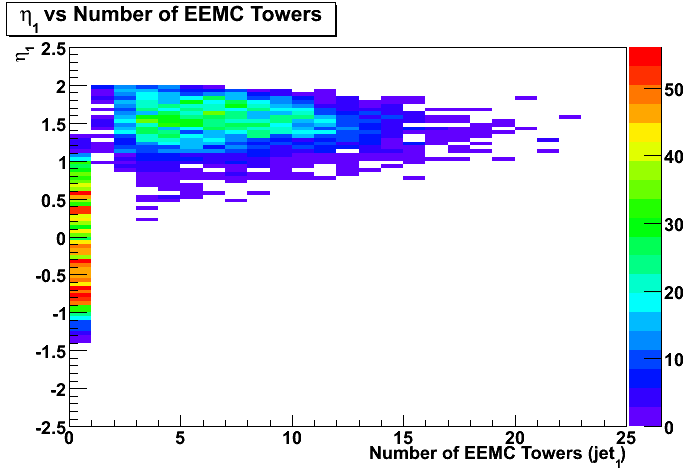
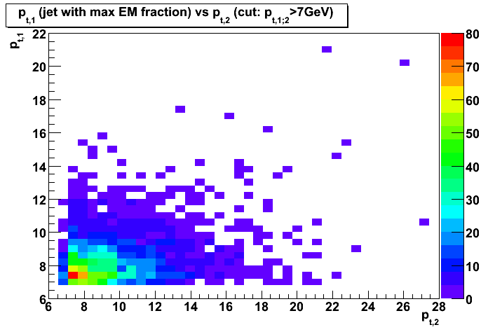
Figure 4: Distribution of transverse momentum, pt1, of the first jet (with maximum EM fraction)
vs transverse momentum, pt2, of the second jet.
Cuts:1-4 applied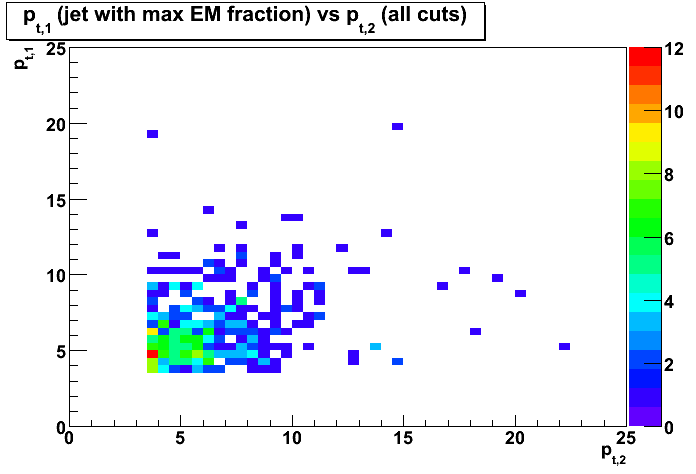
Figure 5: Distribution of mean transverse momentum, < pt1 >, of the first jet (with maximum EM fraction)
vs transverse momentum, pt2, of the second jet.
Cuts:1-4 applied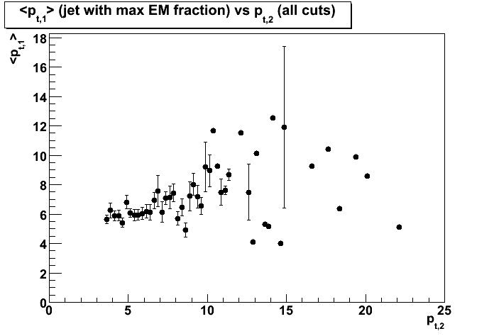
Figure 6: Distribution of pseudorapidity, eta1, of the first jet (with maximum EM fraction)
vs pseudorapidity, eta2, of the second jet.
Cuts:1-4 applied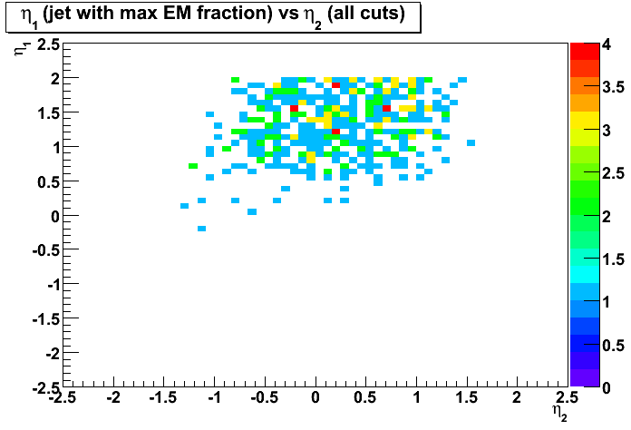
Figure 7: Distribution of azimuthal angle, phi1, of the first jet (with maximum EM fraction)
vs azimuthal angle, phi2, of the second jet.
Cuts:1-4 applied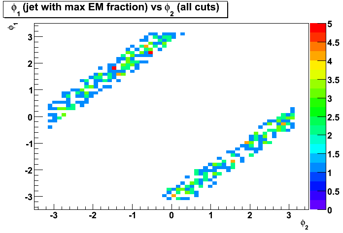
Figure 8: Distribution of transverse momentum, pt1, of the first jet (with maximum EM fraction)
vs transverse energy sum for the EEMC towers associated with this jet.
Cuts:1-4 applied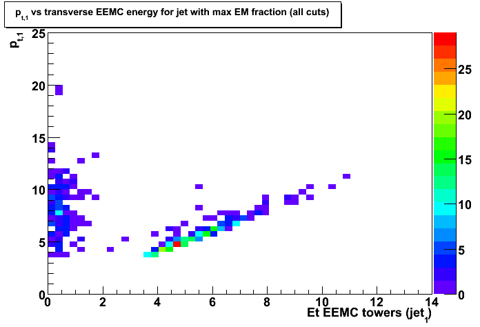
Figure 9: Distribution of transverse momentum, pt1, of the first jet (with maximum EM fraction)
vs transverse momentum, pt2, of the second jet.
Cuts:1-4 + Et(EEMC) > 3.0 GeV

02 Feb

February 2008 posts

2008.02.13 Gamma-jet candidates: EEMC response

Ilya Selyuzhenkov February 13, 2008

Data sample

Gamma-jet selection cuts are discussed here. There are 278 candidates found for runId=7136022.
Transverse momentum distribution for the gamma-jet candidates can be found here.

Vertex z distribution for di-jet and gamma-jet events

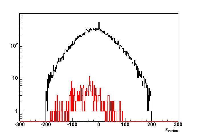
Figure 1: Vertex z distribution.

Red line presents gamma-jet candidates (scaled by x50). Black is for all di-jet events.
Same data on a log scale is here.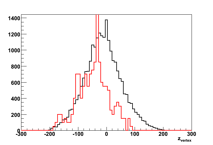
Figure 2: Average vertex z as a function of transverse momentum of the fist jet (with a largest EM energy fraction).
Red is for gamma-jet candidates. Black is for all di-jet events.
Strong deviation from zero for gamma-jet candidates at pt < 5GeV?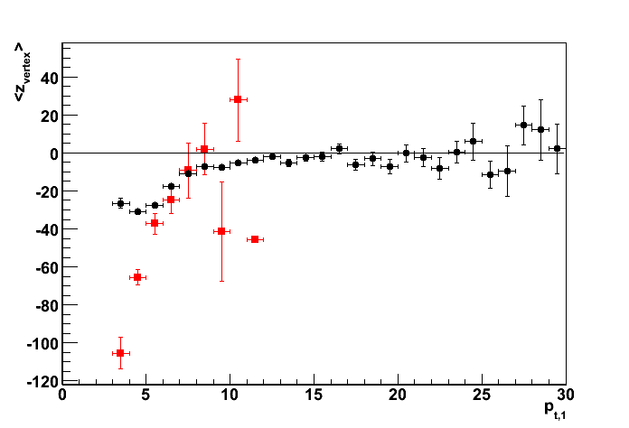

EEMC response for the gamma-jet candidate

EEMC response event by event for all 278 gamma-jet candidate can be found in this pdf file.
Each page shows SMD/Tower energy distribution for a given event:

First row on each page shows SMD response
for the sector which has a maximum energy deposited in the EEMC Tower
(u-plane is on the left, v-plane is on the right).
In the left plot (u-plane energy distribution) numerical values for
pt of the first jet (with maximum EM fraction) and the second jet are given.
In addition, fit results assuming gamma (single Gaussian, red line) or
neutral pion (double Gaussian, blue line ~ red+green) hypotheses are given.
m_{gamma gamma} value (it is shown in the right plot for v-plane).
If m_{gamma gamma} value is negative, then the reconstruction procedure has failed
(for example, no uv-strips intersection found, or tower energy and uv-strips intersection point mismatch, etc).
EEMC response for these "bad" events can be found in this pdf file.

If reconstruction procedure succeded, then
m_{gamma gamma} gives reconstructed invariant mass assuming that two gammas hit the calorimeter.

Figure 3: invariant mass distribution (assuming pi0 hypothesis).

Note, that I'm still working on my fitting algorithm (which is not explained here),
and fit results and the invariant mass distribution will be updated.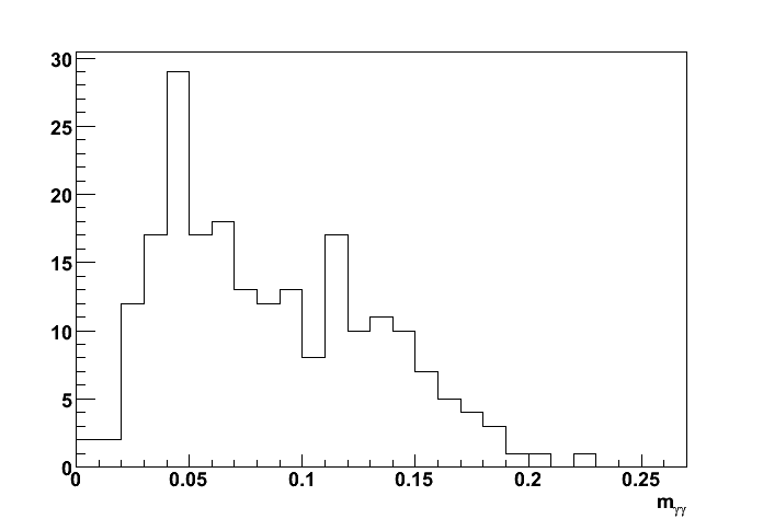
It is also shown the ratio for each u/v plane
of the integrated single Gaussian fit (red line) to the total energy in the plane
(look for "gamma U/V " values on the right v-plane plot).
Second and third rows on each page show the energy deposition in the
tower, pre-shower1, pre-shower2, and post-shower as a function of eta:phi (etaBin:phiBin).
Last row shows the hit distribution in the SMD for all sectors
(u-plane on the left, v-plane of the right).

Playing with a different cuts

Trying to isolate the real gammas which hits the calorimeter,
I have sorted events into different subsets based on the following set of cuts:

EEMC gamma-jet cuts (energetic photon hits EEMC with pt similar or greater to that of the opposite jet)
if (invMass < 0) reject
if (jet2_pt > jet1_pt) reject
if (jet1_pt < 7) reject
if (minFraction < 0.75) reject
(minFraction = gamma U/V - is a fraction of the integrated single Gaussian peak to the total energy in the uv-plane)

Figure 4: Sample gamma-jet candidate EEMC response
(all gamma-jet candidates selected according to these conditions can be found in this pdf file):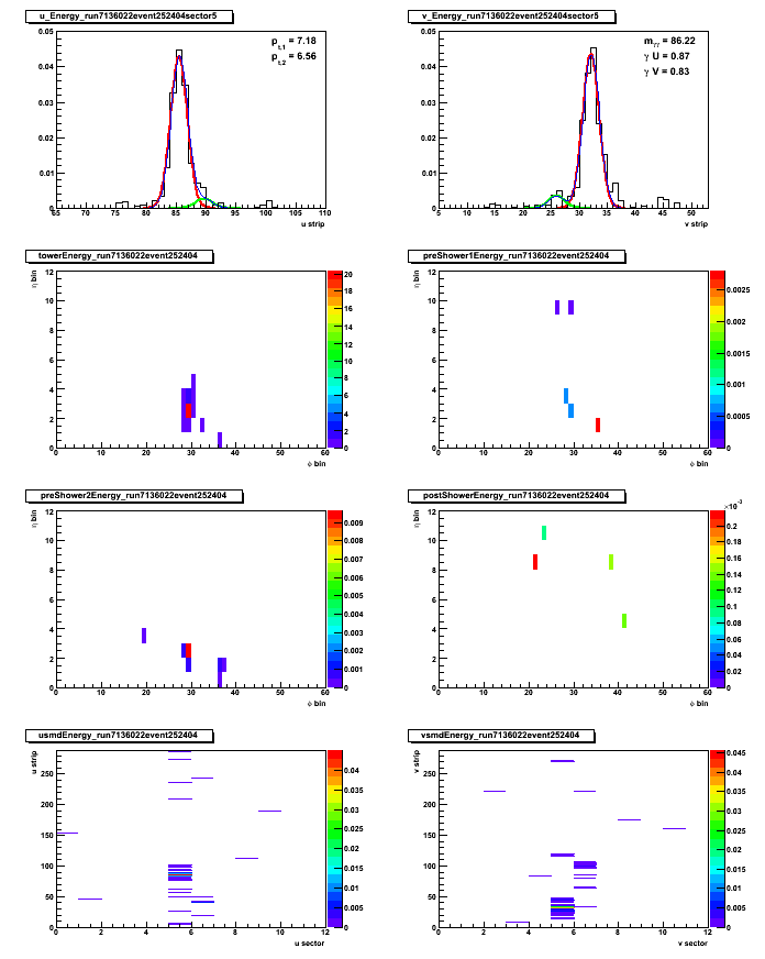
EEMC pi0 cuts:
if (invMass < 0) reject
if (jet2_pt < jet1_pt) reject
if (jet2_pt < 7) reject
if (minFraction < 0.75) reject

Event by event EEMC response for pi0 (di-jet) candidates
selected according to these conditions can be found in this pdf file.

2008.02.20 Gamma-jet candidates: more statistics from jet-trees

Ilya Selyuzhenkov February 20, 2008

Short summary

After processing all available jet-trees for pp2006 (ppProductionLong),
and applying all "gamma-jet" cuts (which are described below):

there are 47K di-jet events selected
for pt1>7GeV there are 5,4K gamma-jet candidates (3,7K with an additional cut of pt1>pt2)
Figure 1: 2,4K events with both pt1, pt2 > 7GeV
721 candidates within a range of pt1>pt2 and both pt1, pt2 > 7 GeV

Data set

jet trees by Murad Sarsour for pp2006 run, number of runs processed: 323
4.7M di-jet events found (no triggerId cuts yet)

Di-jets gross features

Figure 2: Distribution of electromagnetic energy (EM) fraction, R_EM, for di-jet events (number of jets/event = 2).
R_EM = [E_t(endcap)+E_t(barrel)]/E_t(total).
Black histogram is for R_EM1 = max(Ra, Rb), red is for R_EM2 = min(Ra, Rb).
Ra and Rb are EM fraction for jets in the di-jet event.
Same data on a log scale is here.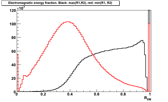

Gamma-jet isolation cuts:

selecting di-jet events with one of the jet dominated by EM energy,
and another one with more hadronic energy:
R_EM1 >0.9 and R_EM2 < 0.9
selecting di-jet events with jets pointing opposite in azimuth:
cos(phi1 - phi2) < -0.9
requiring the number of associated charged tracks with a first jet (with maximum EM fraction) to be less than 2:
nChargeTracks1 < 2
requiring the number of fired EEMC towers associated with a first jet (with maximum EM fraction) to be 1 or 2:
0 < nEEMCtowers1 < 3

Applying gamma-jet isolation cuts

Figure 3: Distribution of eta vs number of EEMC towers for the first jet (with maximum EM fraction).
Cuts:1-3 applied (no 0 < nEEMCtowers1 < 3 cut).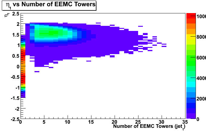
Figure 4: Distribution of transverse momentum, pt1, of the first jet (with maximum EM fraction)
vs transverse momentum, pt2, of the second jet.
Cuts:1-4 applied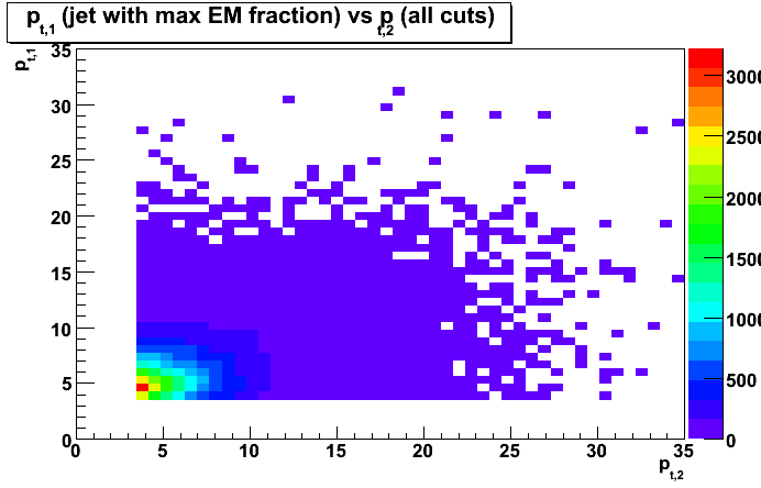
Figure 5: Distribution of mean transverse momentum, < pt1 >, of the first jet (with maximum EM fraction)
vs transverse momentum, pt2, of the second jet.
Cuts:1-4 applied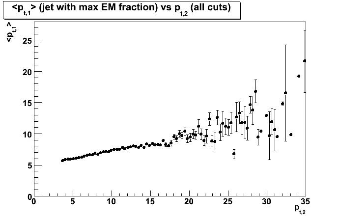
Figure 6: Distribution of pseudorapidity, eta1, of the first jet (with maximum EM fraction)
vs pseudorapidity, eta2, of the second jet.
Cuts:1-4 applied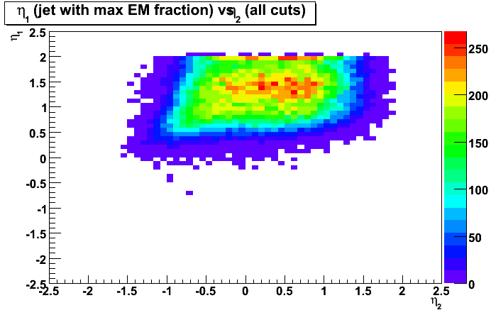
Figure 7: Distribution of azimuthal angle, phi1, of the first jet (with maximum EM fraction)
vs azimuthal angle, phi2, of the second jet.
Cuts:1-4 applied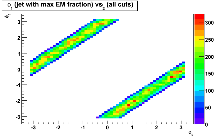
Figure 8: Distribution of transverse momentum, pt1, of the first jet (with maximum EM fraction)
vs transverse energy sum for the EEMC towers associated with this jet.
Cuts:1-4 applied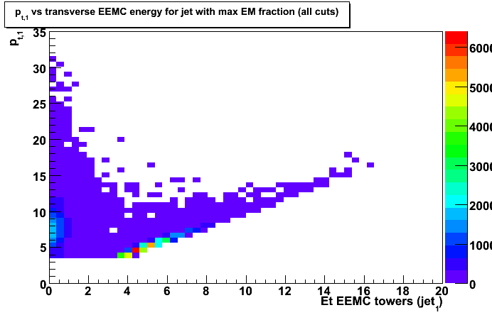
Figure 9: Distribution of transverse momentum, pt1, of the first jet (with maximum EM fraction)
vs transverse momentum, pt2, of the second jet.
Cuts:1-4 + Et(EEMC) > 3.0 GeV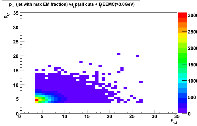

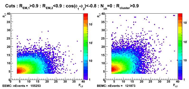
2008.02.27 Tower based clustering algorithm, and EEMC/BEMC candidates

Ilya Selyuzhenkov February 27, 2008

Gamma-jet candidates before applying clustering algorithm

Gamma-jet isolation cuts:

selecting di-jet events with the first jet dominated by EM energy,
and the second one with a large fraction of hadronic energy:
R_EM1 >0.9 and R_EM2 < 0.9
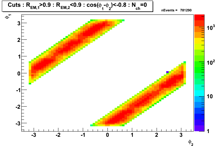
selecting di-jet events with jets pointing opposite in azimuth:
cos(phi1 - phi2) < -0.8
requiring no charge tracks associated with a first jet (jet with a maximum EM fraction):
nCharge1 = 0

Figure 1: Transverse momentum

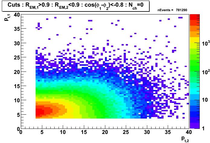
Figure 2: Pseudorapidity

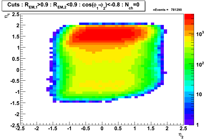
Figure 3: Azimuthal angle

Tower based clustering algorithm

for each gamma-jet candidate finding a tower with a maximum energy
associated with a jet1 (jet with a maximum EM fraction).
Calculating energy of the cluster by finding all adjacent towers and adding their energy together.
Implementing a cut based on cluster energy fraction, R_cluster, where
R_cluster is defined as a ratio of the cluster energy
to the total energy in the calorimeter associated with a jet1.
Note, that with a cut Ncharge1 =0, energy in the calorimeter is equal to the jet energy.

Distribution of cluster energy vs number of towers fired in EEMC/BEMC

Figure 4: R_cluster vs number of towers fired in EEMC (left) and BEMC (right). No pt cuts.

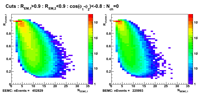
Figure 5: R_cluster vs number of towers fired in EEMC (left) and BEMC (right). Additional cut: pt1>7GeV

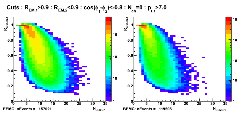
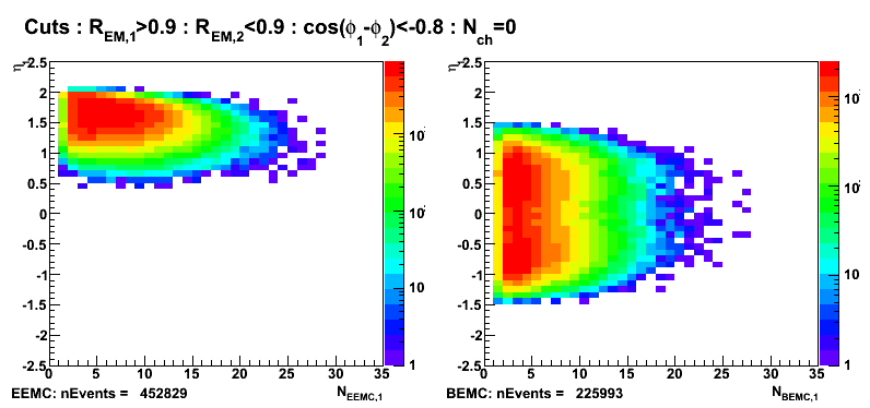
Figure 6: jet1 pseudorapidity vs number of towers fired in EEMC (left) and BEMC (right).

R_cluster>0.9 cut: EEMC vs BEMC gamma-jet candidates

EEMC candidates: nTowerFiredBEMC=0
BEMC candidates: nTowerFiredEEMC=0

Figure 7: Pseudorapidity (left EEMC, right BEMC candidates)

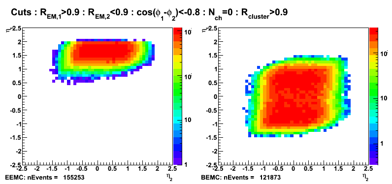
Figure 8: Azimuthal angle (left EEMC, right BEMC candidates)

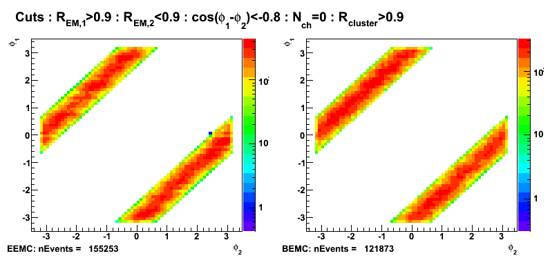
Figure 9: Transverse momentum (left EEMC, right BEMC candidates)

Number of gamma-jet candidates with an addition pt cuts

Figure 10: Transverse momentum (left EEMC, right BEMC candidates): pt1>7GeV

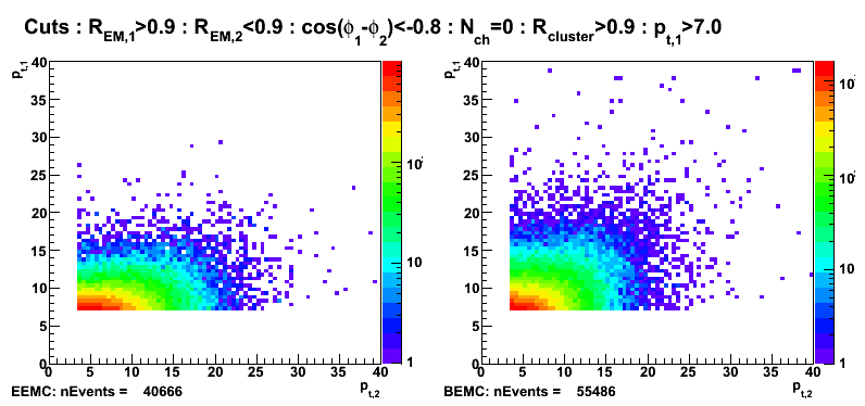
Figure 11: Transverse momentum (left EEMC, right BEMC candidates): pt1>7 and pt2>7

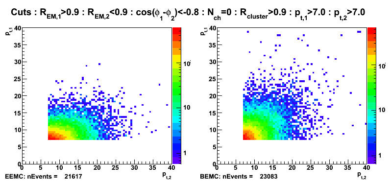
03 Mar

March 2008 posts

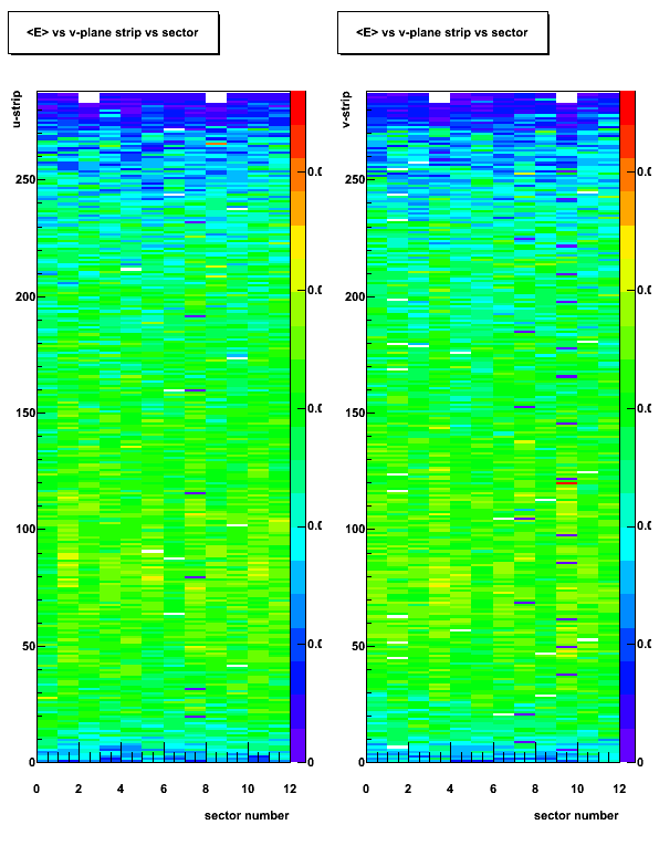
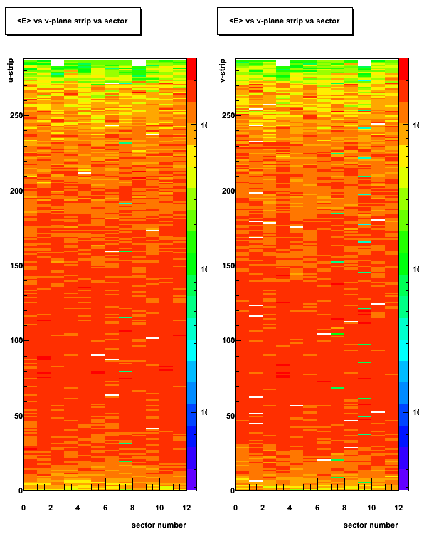
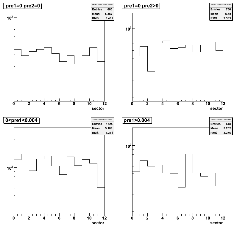
2008.03.03 EEMC SMD: u/v-strip energy distribution

Ilya Selyuzhenkov March 03, 2008

Data set: ppLongitudinal, runId = 7136033.

Some observations/questions:

In general distributions look clean and good
Sectors 7 and 9 for v-plane and sector 7 for u-plane are noise.
Sector 9 has a hot strip (id ~ 120)
In sector 3, strips id=0-5 in v-plane are hot (see figure 2 right, bottom)
Sectors 2 and 8 in u-plane and sectors 3 and 9 in v-plane have missing strips id=283-288?
Strips 288 are always empty?

Figure 1:Average energy E in the strip vs sector and strip number (max < E > = 0.0027)
same figure on a log scale

Figure 2: Average energy E for E>0.02 (max < E > = 0.0682)
Same figure on a log scale

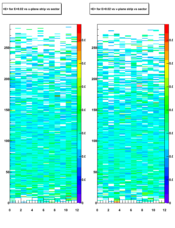
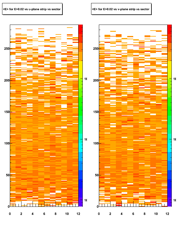
2008.03.12 Gamma-jet candidates: 2-gammas invariant mass and Eemc response

Ilya Selyuzhenkov March 12, 2008

Gamma-jet candidates: 2-gammas invariant

Note: Di-jet transverse momentum distribution for these candidates can be found on figure 11 at this page

Figure 1:Invariant mass distribution for gamma-jet candidates assuming pi0 (2-gammas) hypothesys

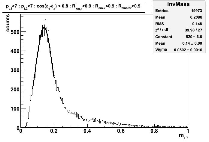
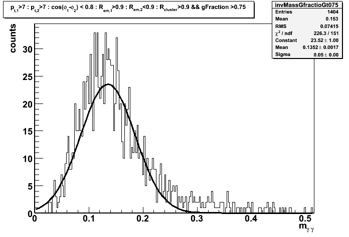
Figure 2:Invariant mass distribution for gamma-jet candidates assuming pi0 (2-gammas) hypothesys
with an additional SMD isolation cut: gammaFraction >0.75
GammaFraction is defined as ratio of the integral
other SMD strips for the first peak to the total energy in the sector

EEMC response for the gamma-jet candidates (gammaFraction >0.75)

pdf file (first 100 events) with event by event EEMC response for the candidates reconstructed into pion mass (gammaFraction >0.75)
pdf file with event by event EEMC response for the candidates not reconstructed into pion mass
(second peak not found), but has a first peak with gammaFraction >0.75.

2008.03.20 Sided residual and chi2 distribution for gamma-jet candidates

Ilya Selyuzhenkov March 20, 2008

Side residual (no pt cut on gamma jet-candidates)

The procedure to discriminate gamma candidate from pions (and other background)
based on the SMD response is described at Pibero's web page.

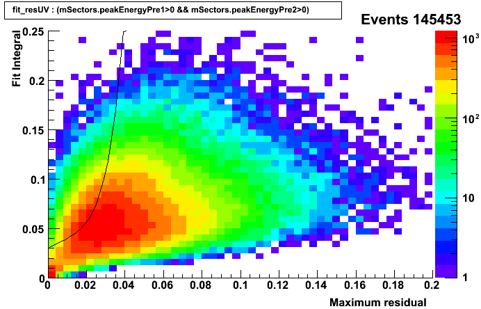
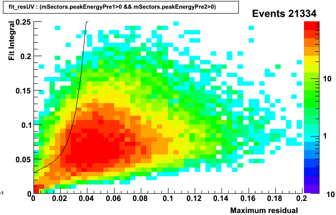
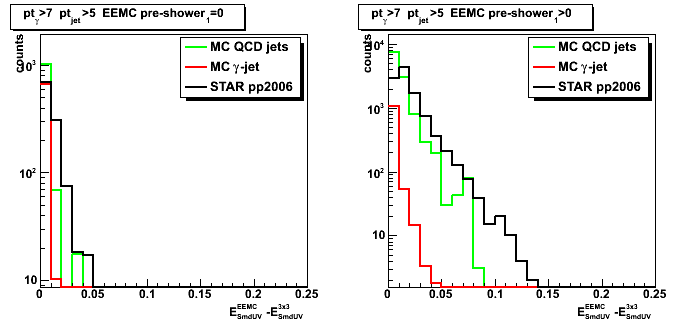
Figure 1: Fit integral vs maximum residual for gamma-jet candidates requesting
no energy deposited in the EEMC pre-shower 1 and 2
(within a 3x3 clusters around tower with a maximum energy).

Black line is defined from MC simulations (see Jason's simulation web page, or Pibero's page above).

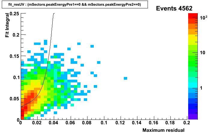
Figure 2: Fit integral vs maximum residual for gamma-jet candidates requesting requesting
no energy deposited in pre-shower 1 cluster and
no energy deposited in post-shower cluster (this cut is not really essential in demonstrating the main idea)

Figure 3: Fit integral vs maximum residual for gamma-jet candidates requesting requesting
non-zero energy deposited in both clusters of pre-shower 1 and 2

Side residual: first and second jet pt are greater than 7GeV

Event by event EEMC response for gamma-jet candidates for the case of
no energy deposited in the EEMC pre-shower 1 and 2 can be found in this pdf file

Figure 4: Fit integral vs maximum residual for gamma-jet candidates requesting
no energy deposited in the EEMC pre-shower 1 and 2

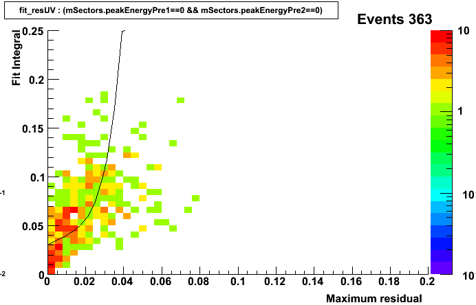
Figure 5: Fit integral vs maximum residual for gamma-jet candidates requesting requesting
no energy deposited in pre-shower 1 cluster and
no energy deposited in post-shower cluster

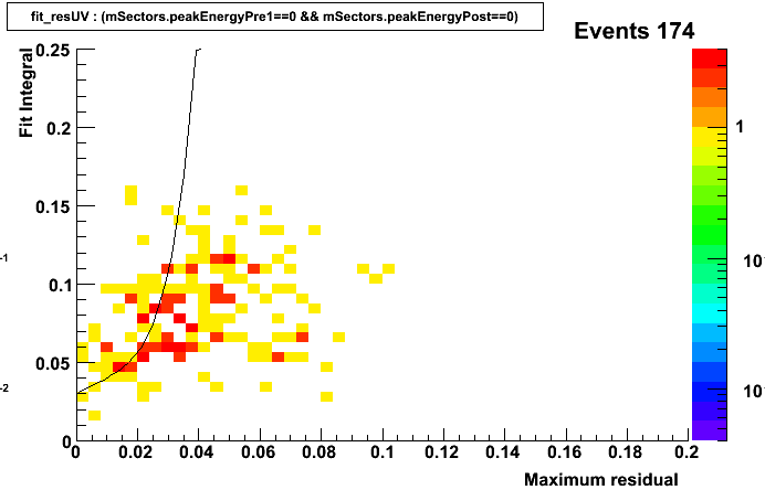
Figure 6: Fit integral vs maximum residual for gamma-jet candidates requesting requesting
non-zero energy deposited in both clusters of pre-shower 1 and 2

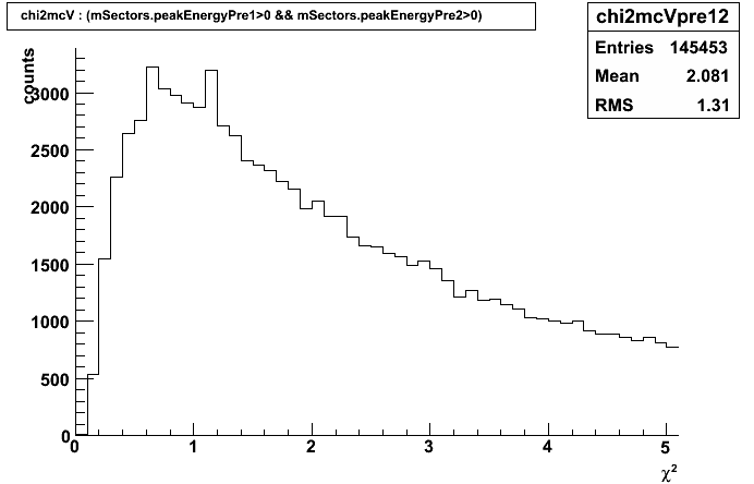
Chi2 distribution for gamma-jet candidates

Monte Carlo shape

Event Monte Carlo shape allows to distinguish gammas from background by cutting at chi2/ndf < 0.5
(although the distribution looks wider than for the case of Will's shape).

Figure 7: Chi2/ndf for gamma-jet candidates using Monte Carlo shape requesting
no energy deposited in both clusters of pre-shower 1 and 2

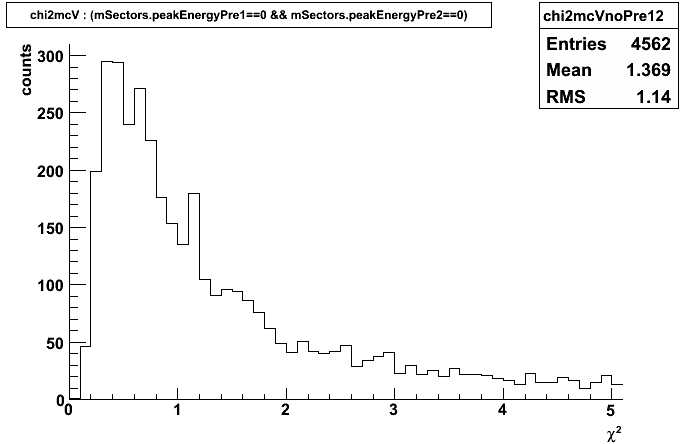
Figure 8: Chi2/ndf for gamma-jet candidates using Monte Carlo shape requesting
non-zero energy deposited in both clusters of pre-shower 1 and 2

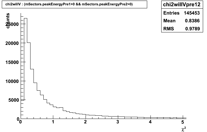
Will''s shape

Less clear where to cut on chi2?

Figure 9: Chi2/ndf for gamma-jet candidates using Monte Carlo shape requesting
no energy deposited in both clusters of pre-shower 1 and 2

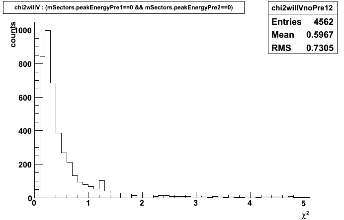
Figure 10: Chi2/ndf for gamma-jet candidates using Monte Carlo shape requesting
non-zero energy deposited in both clusters of pre-shower 1 and 2

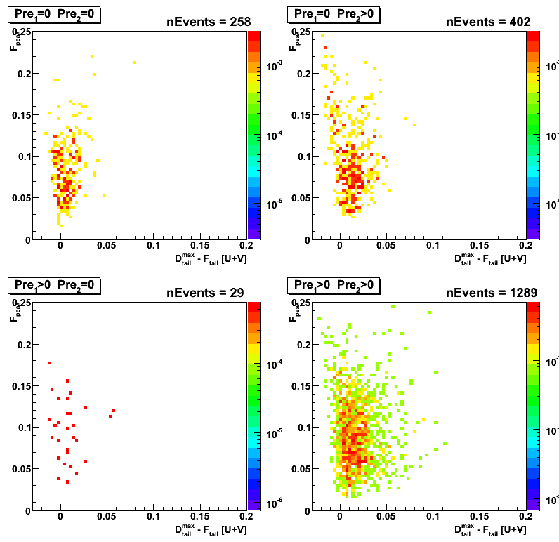
2008.03.26 Sided residual and chi2 distribution for gamma-jet candidates (pre1,2 sorted)

Ilya Selyuzhenkov March 26, 2008

gamma-jet candidates (no pt cut)

Definitions:

F_peak - integral for a fit within [-2,2] strips around SMD u/v peak
D_peak - integral over the data within [-2,2] strips around SMD u/v peak
D_tail^max (D_tail^min) - maximum (minimum) integral over the data tail within +-[3,30] strips from a SMD u/v peak
F_tail is the integral over the fit tail within [3,30] strips from a SMD u/v peak.
Maximum residual = D_tail^max - F_tail

All results are for combined distributions from u and v planes: ([u]+[v])/2
Gamma-jet isolation cuts described here
Additional quality cuts:

Matching between 3x3 tower cluster and u-v high strip intersection
At least 4 strips fired within [-2,2] strips from a peak

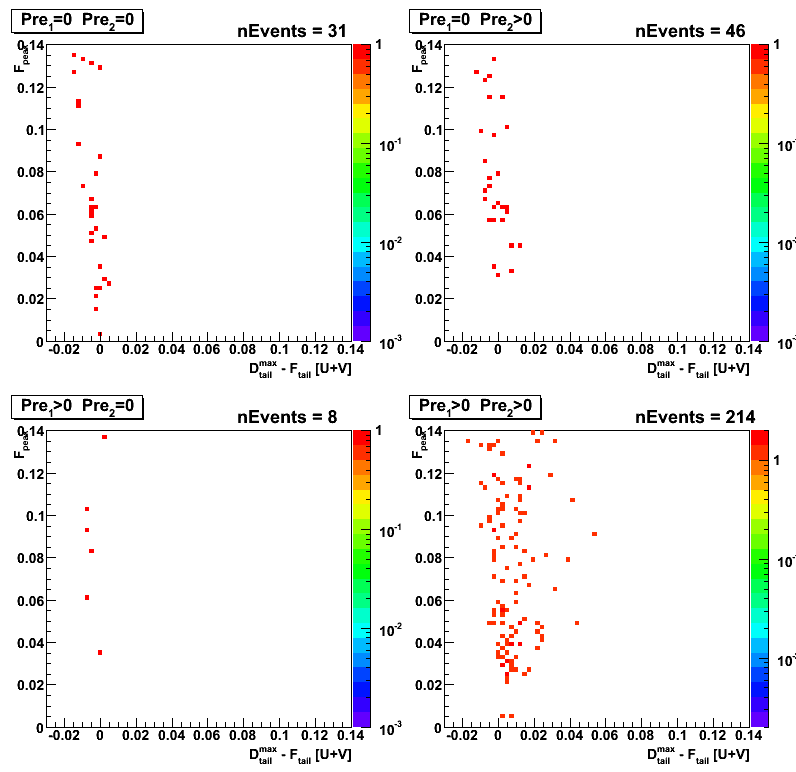
Figure 1: F_peak vs maximum residual
for various cuts on energy deposited in the EEMC pre-shower 1 and 2
(within a 3x3 clusters around tower with a maximum energy).

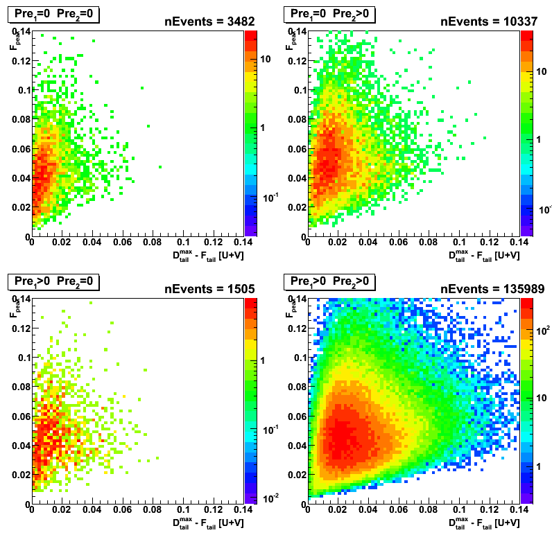
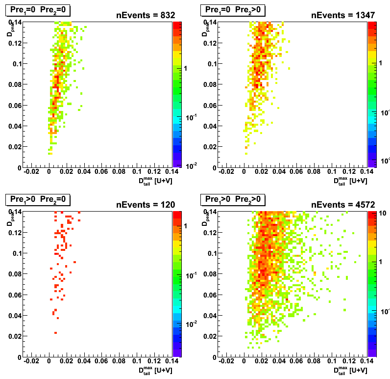
Figure 2: F_data vs D_tail^max
Note:This plot is fit independend (only the peak position is defined based on the fit)

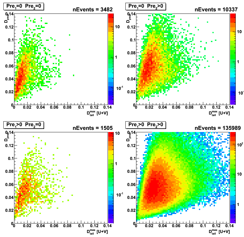
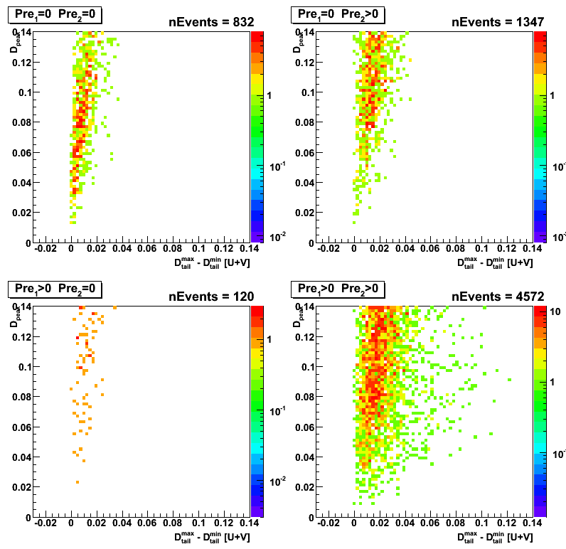
Figure 3: F_data vs D_tail^max-D_tail^max

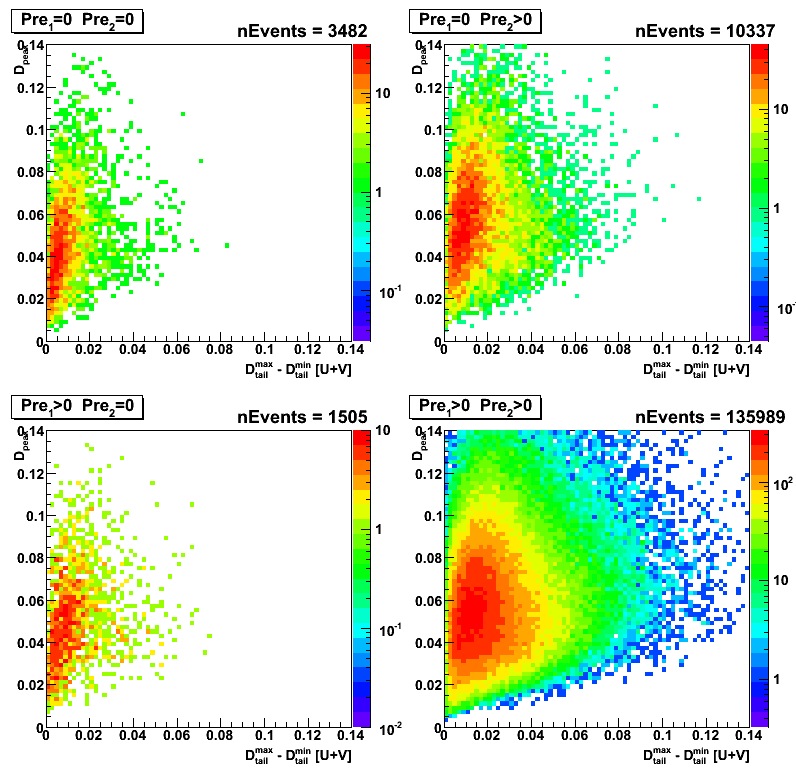
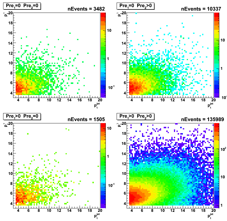
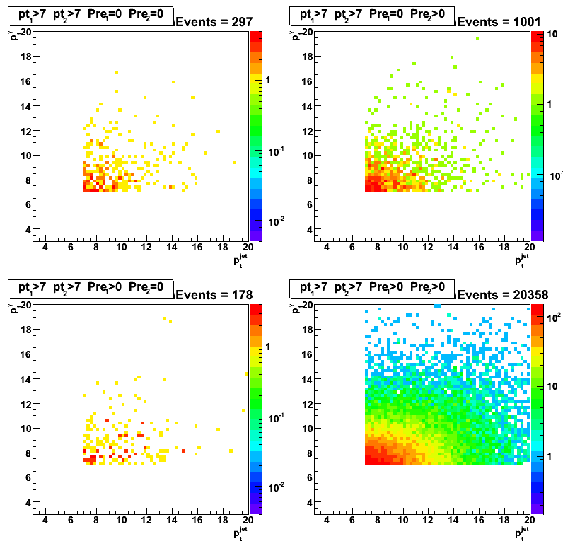
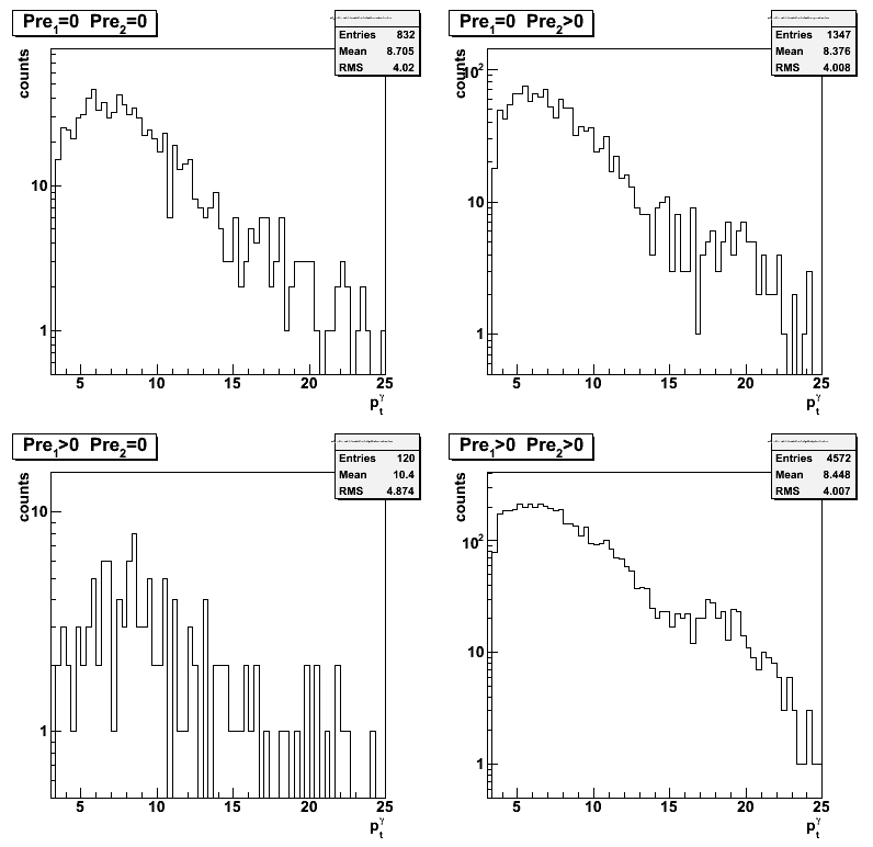
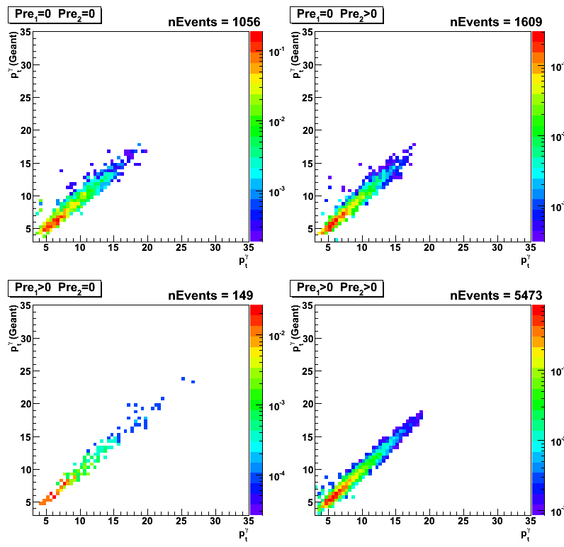
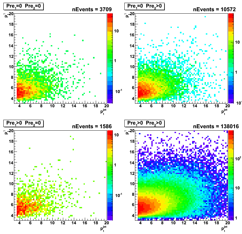
Figure 4: Gamma transverse momentum vs jet transverse momentum

gamma-jet candidates: pt > 7GeV

Figure 5: F_peak vs maximum residual
for various cuts on energy deposited in the EEMC pre-shower 1 and 2
(within a 3x3 clusters around tower with a maximum energy).

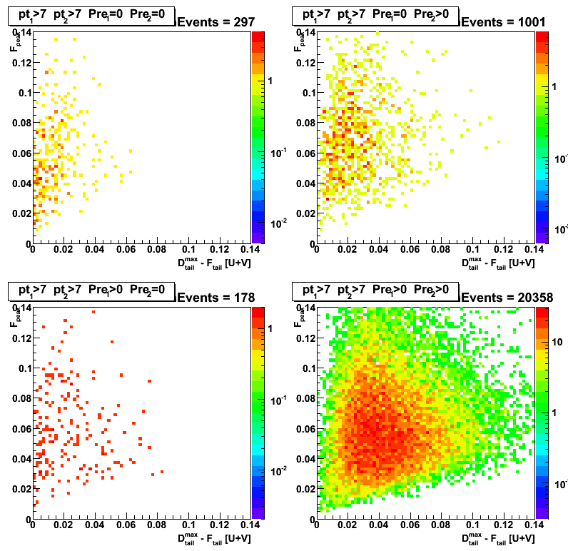
Figure 6: F_data vs D_tail^max
Note:This plot is fit independend (only the peak position is defined based on the fit)

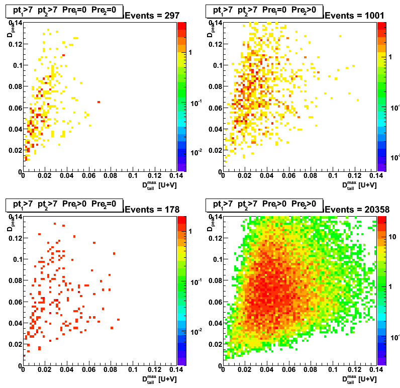
Figure 7: F_data vs D_tail^max-D_tail^max

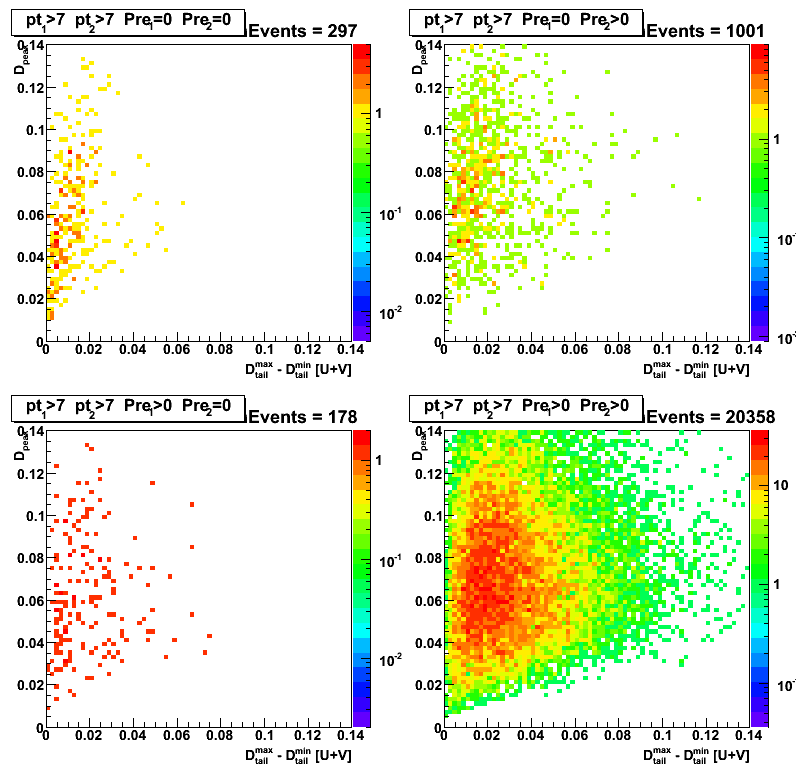
Figure 8: Gamma transverse momentum vs jet transverse momentum

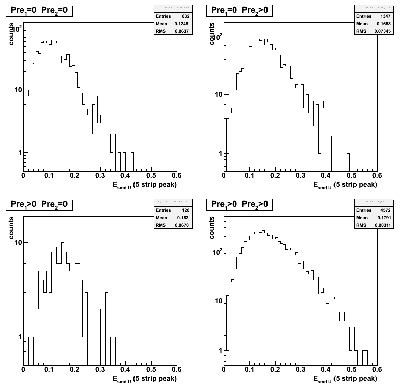
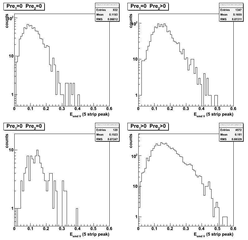
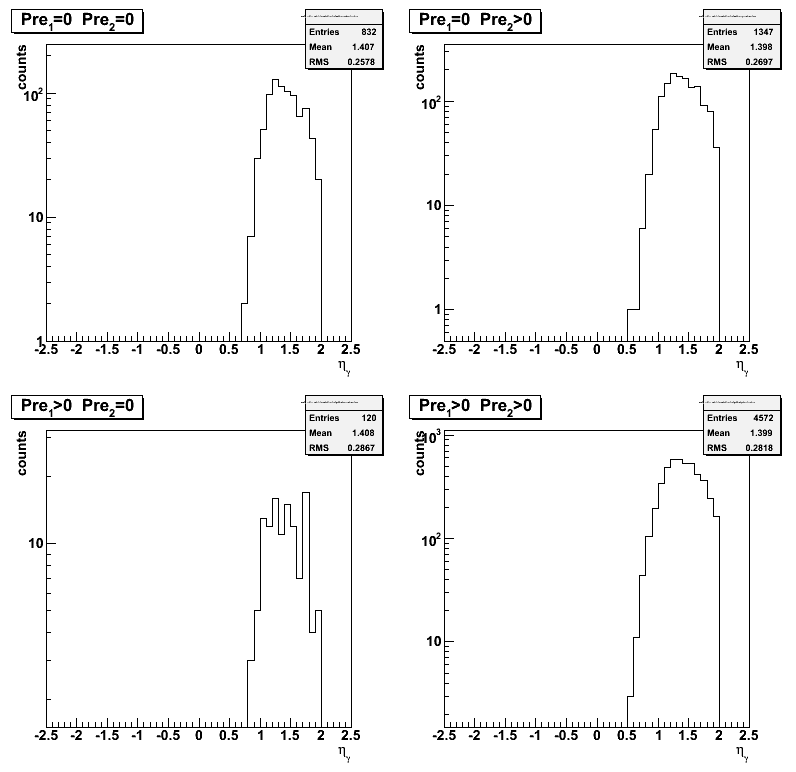
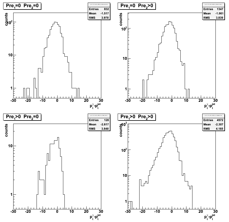
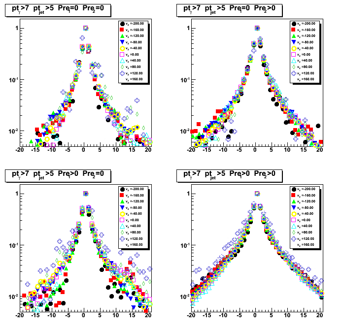
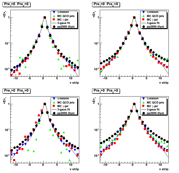
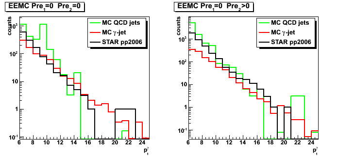
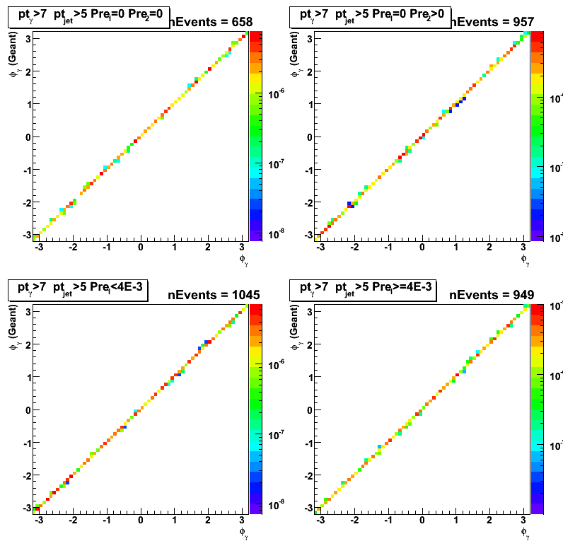
gamma-jet candidates: eta, phi, and max[u,v] strip distributions (no pt cuts)

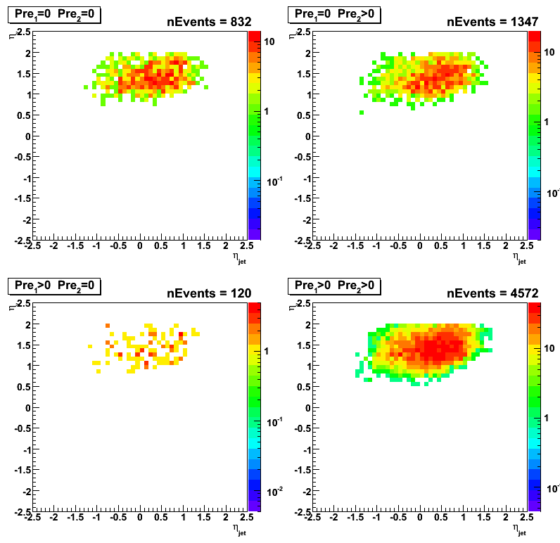
Figure 9: Gamma pseudorapidity vs jet pseudorapidity

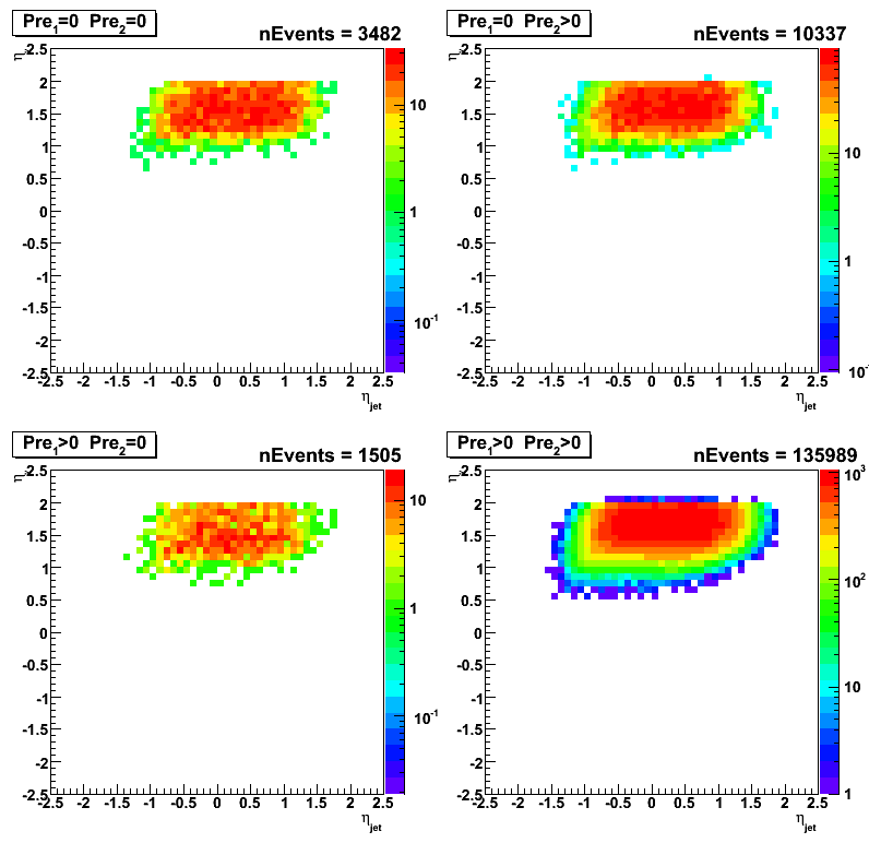
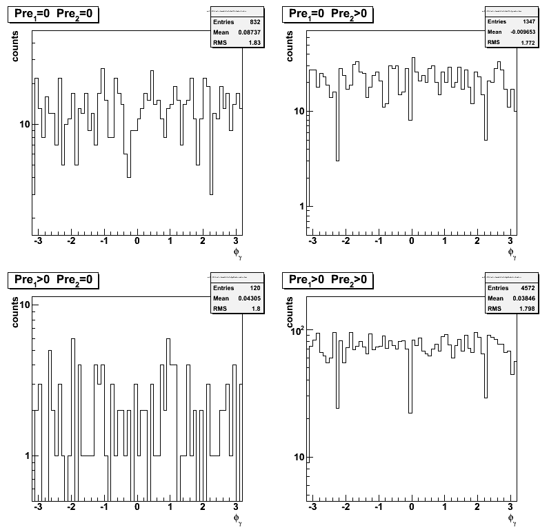
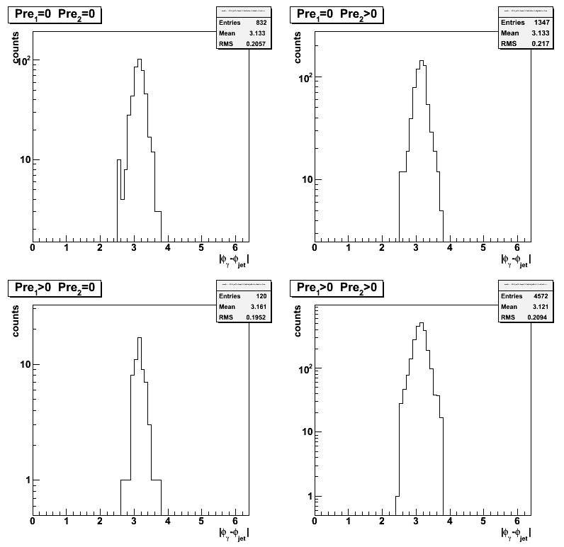
Figure 10: Gamma azimuthal angle vs jet azimuthal angle
Note: for the case of Pre1>1 && Pre2==0 there is an enhancement around phi_gamma = 0?

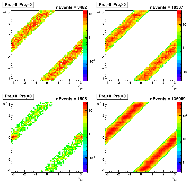
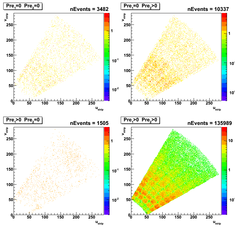
Figure 11: maximum strip in v-plane vs maximum strip in u-plane

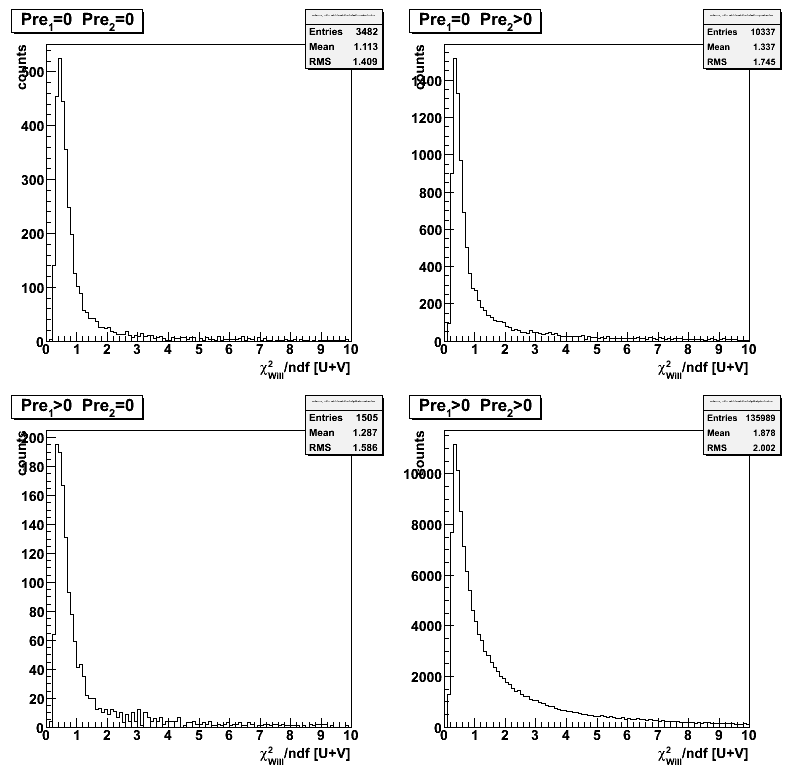
Chi2 distribution for gamma-jet candidates (no pt cuts)

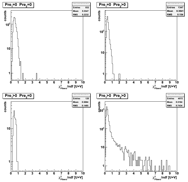
Figure 12:Chi2/ndf for gamma-jet candidates using Monte Carlo shape (combined for [u+v]/2 plane )

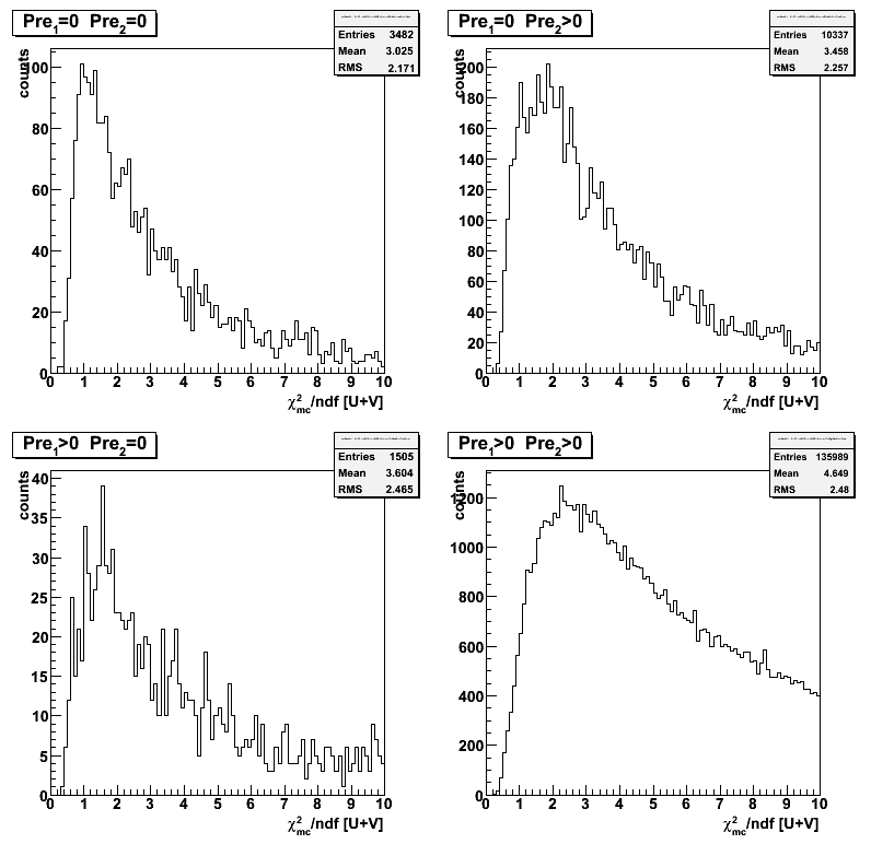
Figure 13:Chi2/ndf for gamma-jet candidates (combined for [u+v]/2 plane ) using Will's shape

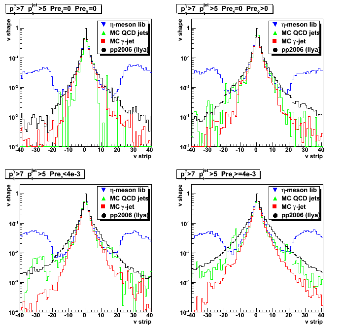
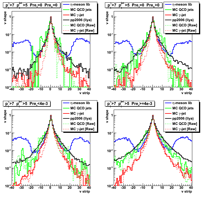
2008.03.28 EEMC SMD shapes: gamma's from gamma-jets (data), MC, and eta-meson analysis

Ilya Selyuzhenkov March 28, 2008

Some observations:

SMD data-driven shapes from different analysis are in a good agreement (Figure 1, upper left plot)
Overall MC shape is too narrow compared to the data shapes (Figure 1, upper left plot)
Shapes are similar with or without gamma-jet 7GeV pt cut (compare Figures 1 and 2),
what may indicate that shape is independent on energy (at least within our kinematic limits).
Data-driven and MC shapes are getting close to each other (Figure 4, upper left plot)
when requiring no energy above threshold in both preshower layers and
with suppressed contribution from pi0 background.
The latter is achieved by using the information on
reconstructed invariant mass of 2gamma candidates (compare Figure 3 and 4).
One interpretation of this can be that in Monte Carlo simulations
the contribution from the material in front of the detector is underestimated
Energy distribution for each strip in the SMD peak does not looks like a Gaussian (Figure 5),
what makes very difficult to interpret results obtained from chi2 analysis (Figure 6-8).
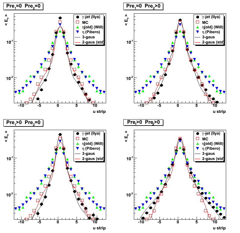
Triple Gaussian fit gives a better description of the data shapes,
compared to the double Gaussian function (compare red and black lines on Figure 1-4)

Figure 1: EEMC SMD shape comparison for various preshower cuts
(black points shows u-plane shape only, v-plane results can be found here)

Figure 2: EEMC SMD shape comparison for various preshower cuts with gamma-jet pt cut of 7GeV
(black points shows u-plane shape only, v-plane results can be found here)

Figure 3: Shapes with an additional cut on 2-gamma candidates within pi0 invariant mass range.
Sample invariant mass distribution using "simple" pi0 finder can be found here
(black points shows u-plane shape only, v-plane results can be found here)

Figure 4: Shapes for the candidates when "simple" pi0 finder failed to find a second peak
(black points shows u-plane shape only, v-plane results can be found here)

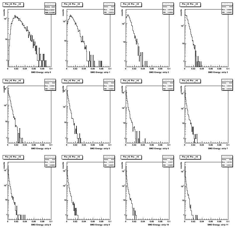
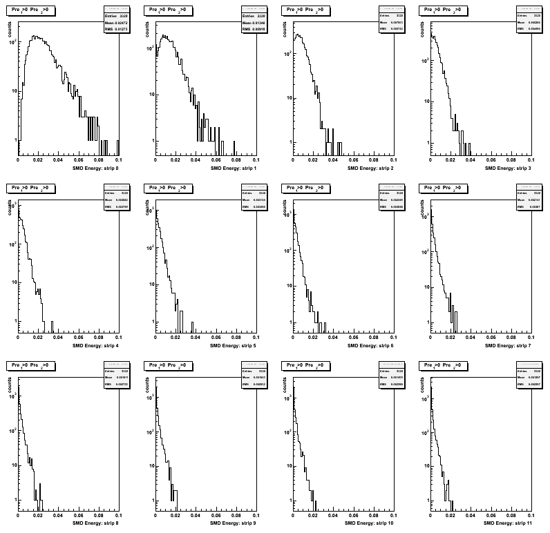
Figure 5: Strip by strip SMD energy distribution.
Only 12 strips from the right side of the maximum are shown.
Zero strip (first upper left plot) corresponds to the high strip in the shape
Note, that already at the 3rd strip from a peak,
RMS values are comparable to those for a mean, and for a higher strips numbers RMS starts to be bigger that mean.
(results for u-plane only, v-plane results can be found here)

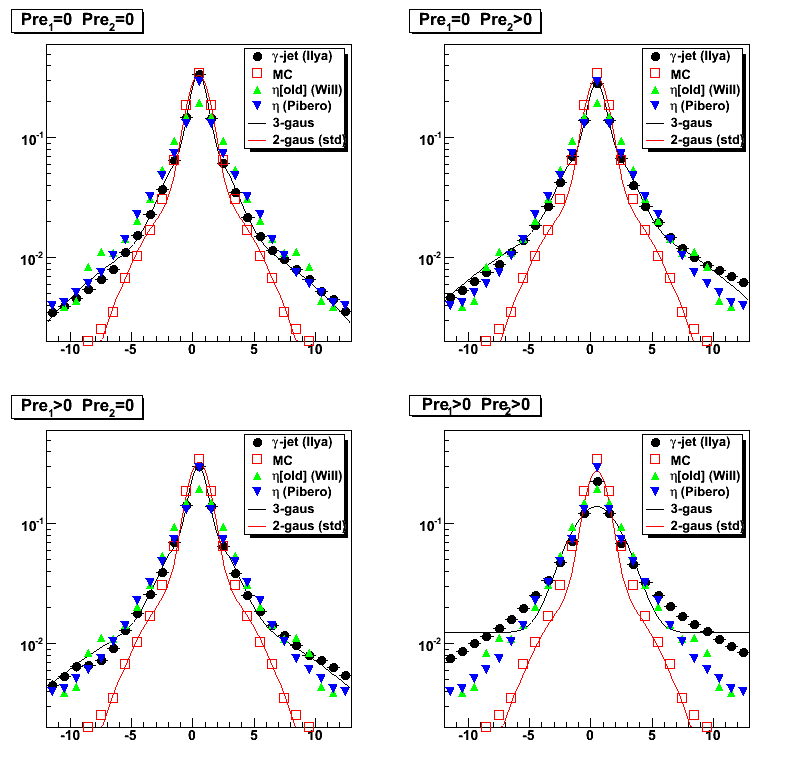
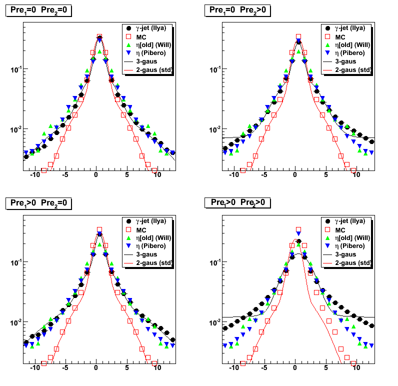
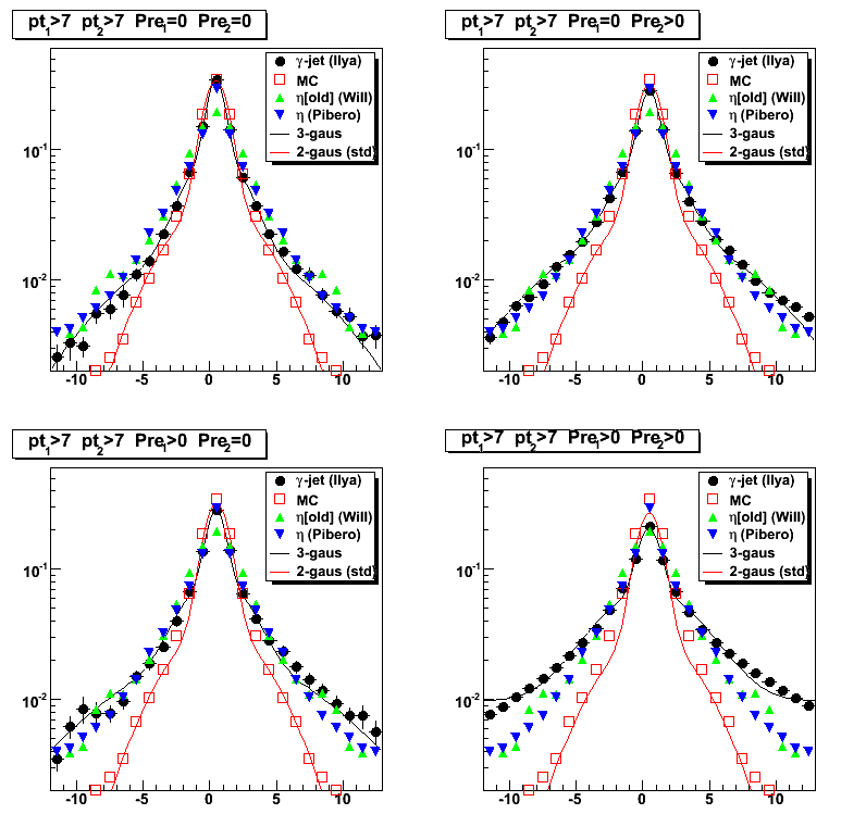
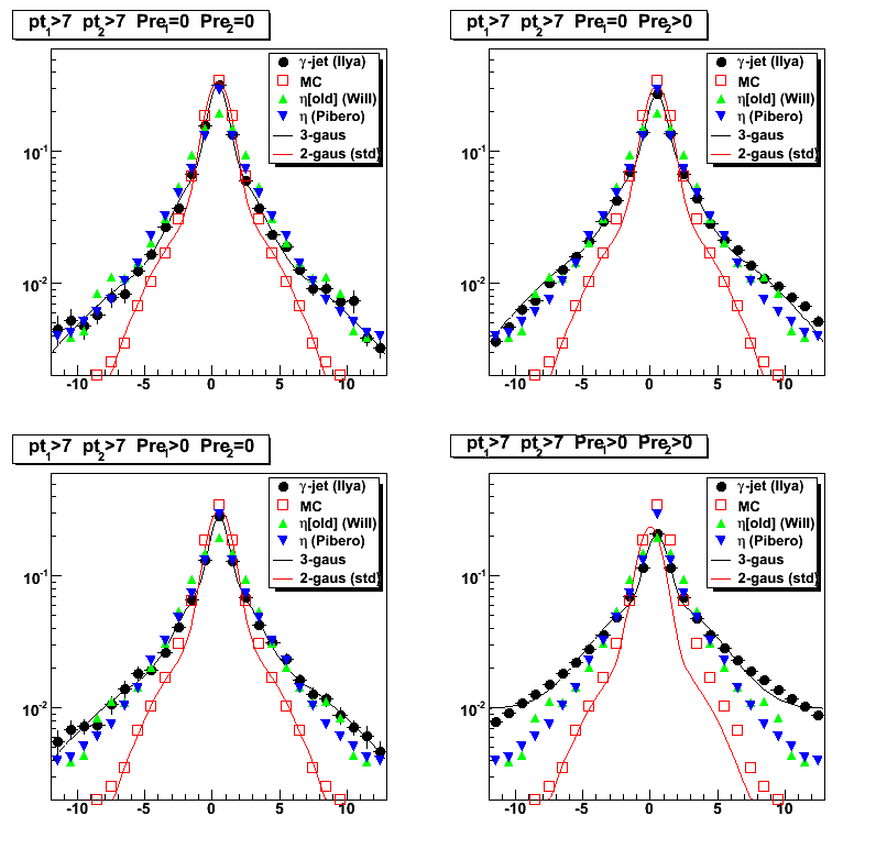
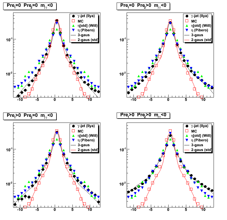
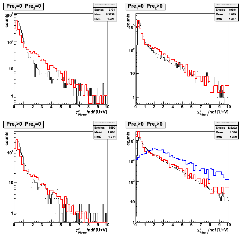
Comparing chi2 distributions for gamma-jet candidates using MC, Will, and Pibero's shapes

Results for side residual (together with pt, eta, phi distributions) for gamma-jet candidates can be found at this web page

Red histograms on Figures 6-8 shows chi2 distribution from MC-photons (normalized at chi2=1.4)
Blue histograms on Figures 6-8 shows chi2 distribution from MC-pions (normalized at chi2=1.4)

Figure 6: Chi2/ndf for gamma-jet candidates using Monte Carlo shape

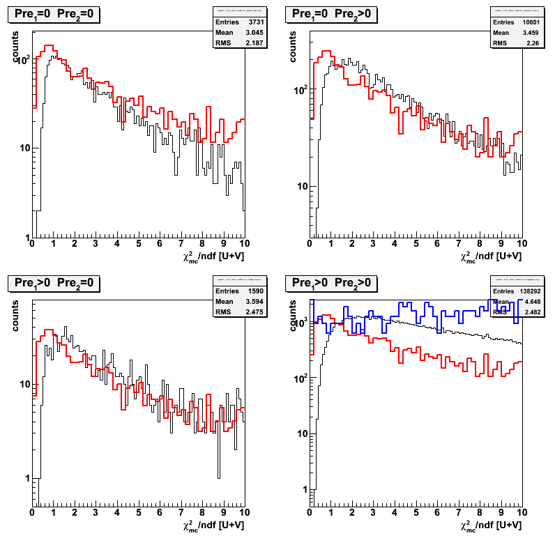
Figure 7: Chi2/ndf for gamma-jet candidates using Will's shape (derived from eta candidates based on Weihong's pi0-finder)

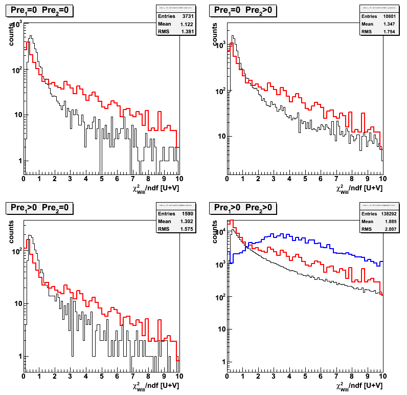
Figure 8: Chi2/ndf for gamma-jet candidates using Pibero's shape (derived from eta candidates)

04 Apr

April 2008 posts

2008.04.02 EEMC SMD shapes: data-driven (eta, gamma-jet) vs Monte Carlo (single gamma, gamma-jet)

Ilya Selyuzhenkov April 02, 2008

Some observations:

SMD data-driven shapes from eta-meson and gamma-jet studies
are in a good agreement for different preshower conditions
(compage Fig.1 green circles/triangles in upper-left/bottom-right plots)
single gamma MC shapes show preshower dependance,
but they are still narrower compared to the data shapes
(compare Fig.1 green circles vs blue open squares)
MC shapes for gamma-jet and single gamma are consistent (Fig.1, bottom right plot)

Figure 1: EEMC SMD shape comparison for various preshower cuts
Note:Only MC gamma-jet shape (open red squares) is the same on all plots

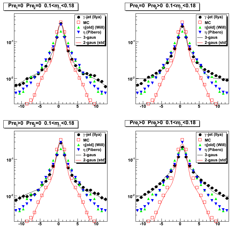
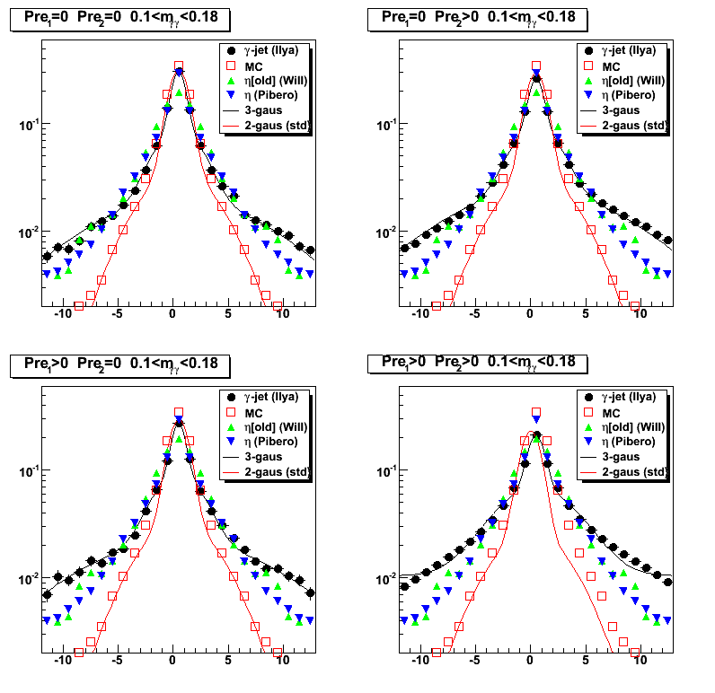
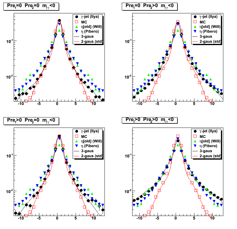
2008.04.02 Sided residual: Using data driven gamma-jet shape (3 gaussian fit)

Ilya Selyuzhenkov April 02, 2008

Figure 1: Side residual for various cuts on energy deposited in the EEMC pre-shower 1 and 2
No EEMC SMD based cuts

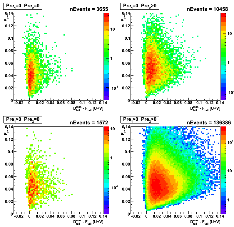
Figure 2: Side residual for various cuts on energy deposited in the EEMC pre-shower 1 and 2
"Simple" pi0 finder can not find a second peak

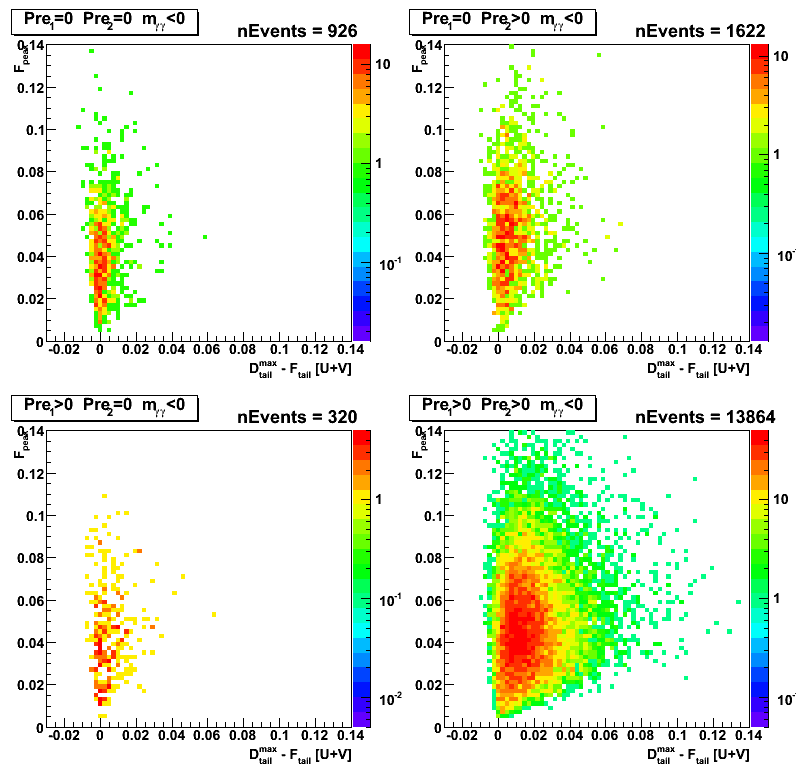
Figure 3: Side residual for various cuts on energy deposited in the EEMC pre-shower 1 and 2
"Simple" pi0 finder reconstruct the invarian mass within [0.1,0.18] range

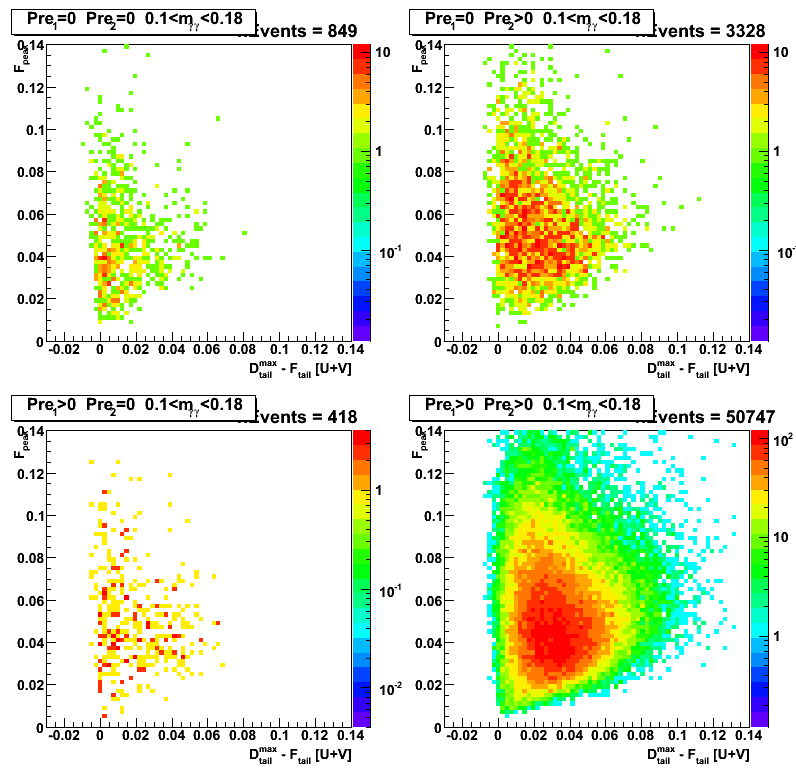
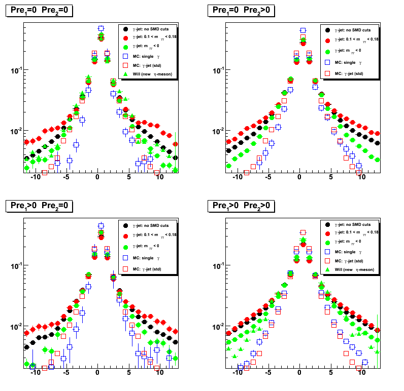
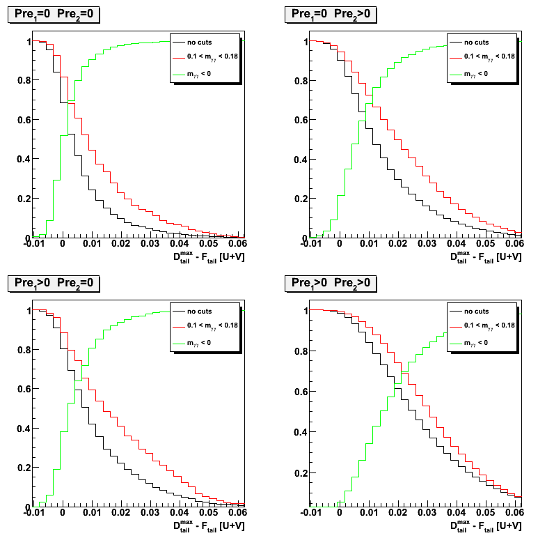
Figure 4: Side residual distribution (Projection for side residual in Figs.1-3 on vertical axis)

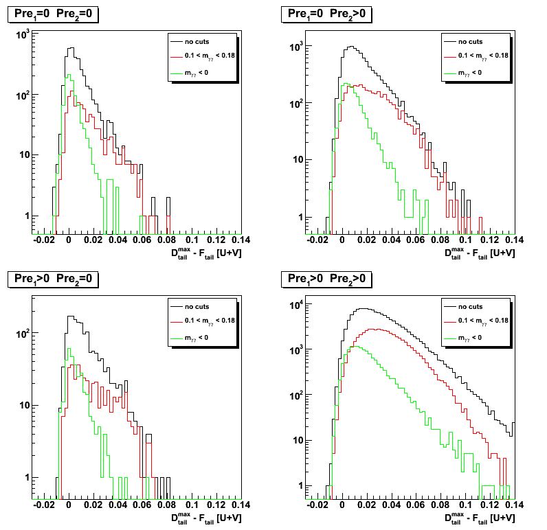
Figure 5: Signal (green: m < 0) vs background (black, red) separation

2008.04.02 Sided residual: single gamma Monte-Carlo simulations

Ilya Selyuzhenkov April 02, 2008

Side residual: single gamma Monte-Carlo simulations

Figure 1: Side residual for various cuts on energy deposited in the EEMC pre-shower 1 and 2
No EEMC SMD based cuts

2008.04.03 chi2-shape subtraction for different Preshower conditions

Ilya Selyuzhenkov April 03, 2008

Request from Hal Spinka:

Hi Ilya,

I think you gave up on the chi-squared method too quickly, and am sorry I missed the phone meeting last week. So, I would like to make a request that will hopefully take a minimal amount of your time to show that all is okay. Then, if there is a delay in getting the sided residual information out and into the beam use request, you can still fall back on the chi-squared method.

In your March 28 posting, Figure 8 at the bottom, I would like to get numerical values for the events per bin for the black curves. I won't use the preshower1>0 and preshower2=0 data, so those you don't need to send. Also, I won't use the red or blue curve information.

I think your problem has been that you normalized your curves at chi-squared/ndf = 1.4 instead of the peak. What I plan to do is to normalize the (pre1=0, pre2=0) to the (pre1=0, pre2>0) data in the peak and subtract. The (pre1=0, pre2=0) set should have some single photons, but also some multiple photons. The (pre1=0, pre2>0) should also have single photons, and more multiple photons, since the chance that one of them will convert is larger. The difference should look roughly like your blue curve, though perhaps not exactly if Pibero's mean shower shape is not perfect (which it isn't). I will do the same thing with taking the difference between (pre1>0, pre2>0) and (pre1=0, pre2=0), and again the difference should look roughly like your blue curve. The (pre1>0, pre2>0) data should have even larger fraction of multiple photons than either of the other two data sets. I would expect the two difference curves to look approximately the same.

Hope this is possible for you to do. Since our reduced chi-squared curve looks so much like the one from CDF, I am pretty confident that we are okay, but this should be checked to convince people that we are not doing anything terribly wrong.

Reply by Ilya:

Dear Hal,

I have tried to implement your idea and produce a figure attached.

There are 4 plots in it:

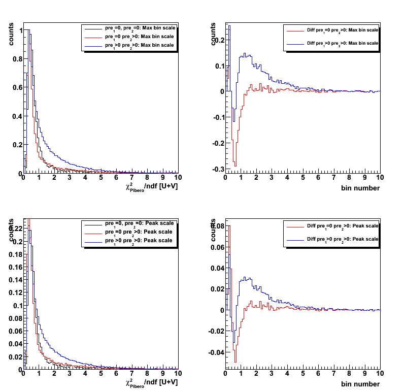
1. Upper left plot shows normalized to unity (at maximum) chi2 distribution (obtained with Pibero shape for gamma-jet candidates) for a different pre1, pre2 conditions

2. Upper right plot shows bin-by-bin difference: a) between normalized chi2 for pre1=0, pre2>0 and pre1=0, pre2=0 (red) and b) between normalized chi2 for pre1>0, pre2>0 and pre1=0, pre2=0 (blue)

3. Bottom left Same as upper right, but normalization were done based on the integral within [-4,4] bins around maximum.

4. Bottom right Same as for upper right, but with a different normalization ([-4,4] bins around maximum)

I have also tried to normalized by the total integral, but the results looks similar.

Figure 1: See description above

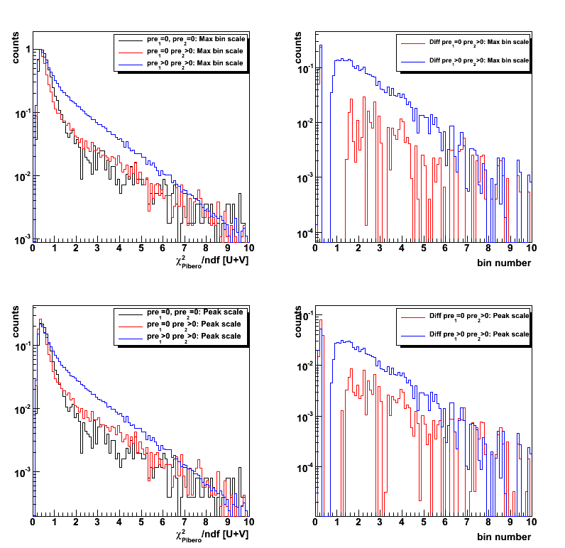
Figure 2: Same without log scale (See description above)

2008.04.09 Applying gamma-jet reconstruction algorithm for gamma-jet simulated events

Ilya Selyuzhenkov April 09, 2008

Data sample:
Monte-Carlo gamma-jet sample for partonic pt range of 5-7, 7-9, 9-11,11-15, 15-25, 25-35 GeV.

Analysis: Simulated MuDst files were first processed through jet finder algorithm (thanks to Renee Fatemi),
and later analyzed by applying gamma-jet isolation cuts (see this link for details) and studying EEMC SMD response (see below).
To test the algorithm, Geant records were not used in this analysis.
Further studies based on Geant records (yield estimates, etc) are ongoing.

EESMD shapes comparison

Figure 1:Comparison between shower shape profile for data and MC.
Black circles shows results for MC gamma-jet sample (all partonic pt).
For v-plane results see this figure

Correlation between gamma and jet pt, eta, phi

Figure 2:Gamma vs jet transverse momentum.

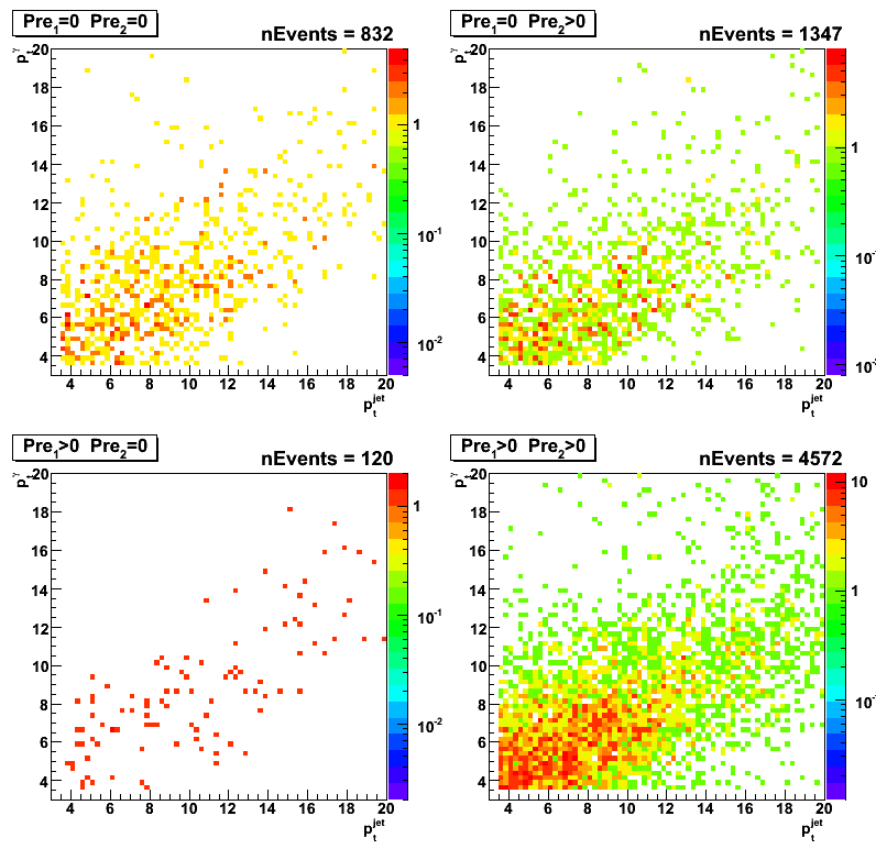
Figure 3:Gamma vs jet azimuthal angle.

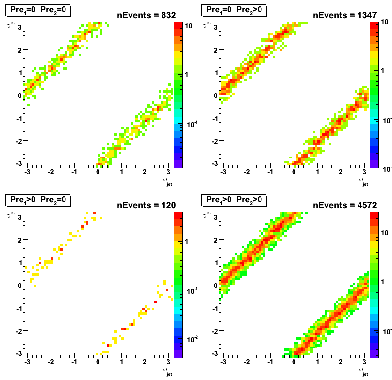
Figure 4:Gamma vs jet pseudo-rapidity.

Results from maximum sided residua study

Definitions for F_peak, D_peak, D_tail^max (D_tail^min) can be found here

Figure 5:F_peak vs maximum residual
for various cuts on energy deposited in the EEMC pre-shower 1 and 2
(within a 3x3 clusters around tower with a maximum energy).
Shower shape used to fit data is fixed to the shape from the previous gamma-jet study of real events
(see black point on Fig.1 [upper left plot] at this page)

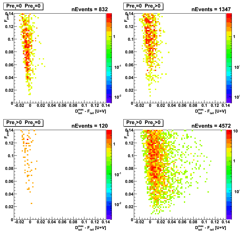
Figure 6: F_peak vs D_tail^max: click here
Figure 7: F_peak vs D_tail^max-D_tail^min: click here

Postshower to SMD[uv] energy ratio

Figure 8:Logarithmic fraction of energy in post shower (3x3 cluster) to the total energy in SMD u- and v-planes

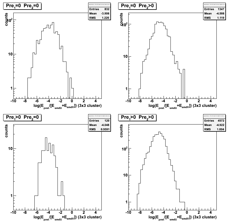
Figure 8a:
Same as figure 8, but for gamma-jet candidates from the real data (no pt cuts).
Logarithmic fraction of energy in post shower (3x3 cluster) to the total energy in SMD u- and v-planes

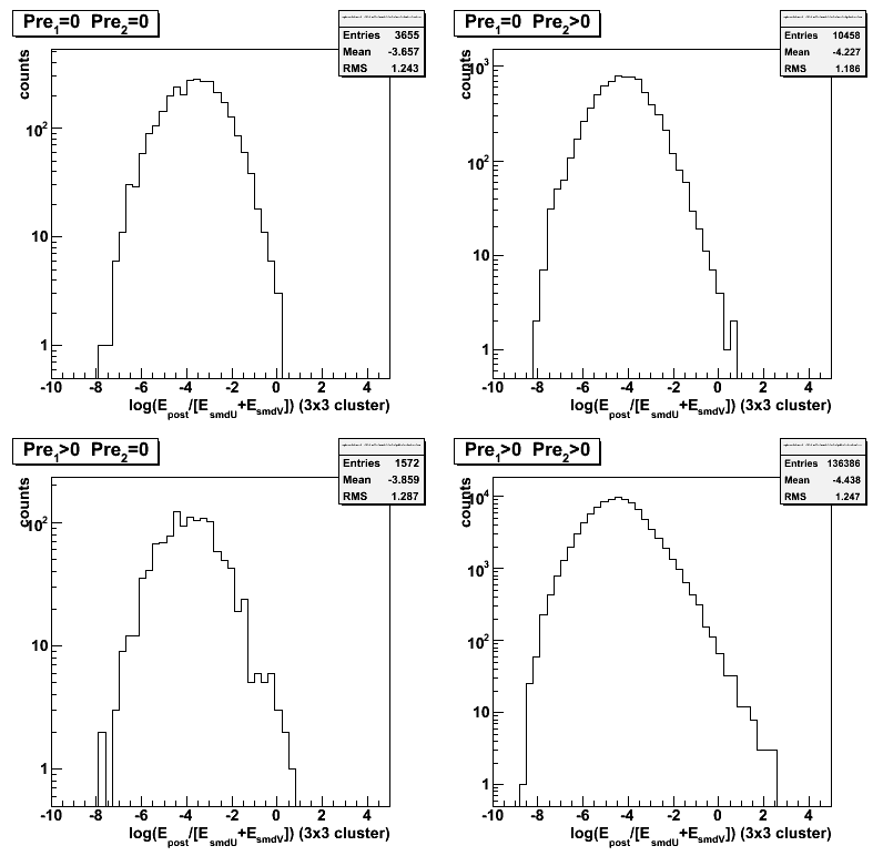
Figure 8b:
Comparison between gamma-jet candidates from data with different preshower conditions.
Points are normalized in peak to the case of pre1 > 0, pre2 > 0
Logarithmic fraction of energy in post shower (3x3 cluster) to the total energy in SMD u- and v-planes

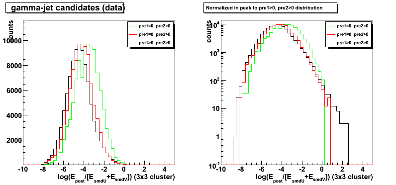
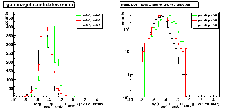
Figure 8c:
Comparison between gamma-jet candidates from Monte-Carlo simulations with different preshower conditions.
Points are normalized in peak to the case of pre1 > 0, pre2 > 0
Logarithmic fraction of energy in post shower (3x3 cluster) to the total energy in SMD u- and v-planes

Additional QA plots

Figure 9: Jet neutral energy fraction
Figure 10: High v-strip vs u-strip
Figure 11: energy post shower (3x3 cluster)
Figure 12: Peak energy SMD-u
Figure 13: Peak energy SMD-v
Figure 14: Gamma phi
Figure 15: Gamma pt
Figure 16: Gamma eta
Figure 17: Delta gamma-jet pt
Figure 18: Delta gamma-jet eta
Figure 19: Delta gamma-jet phi

chi2 distributions

Figure 20:chi2 distribution using "standard" MC shape

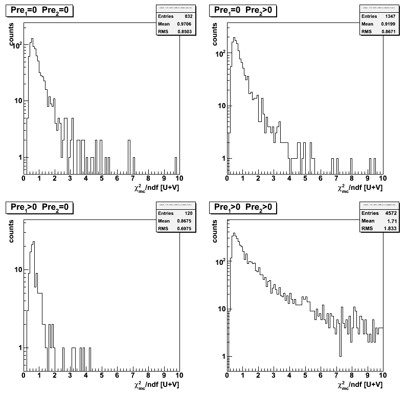
Figure 21:chi2 distribution using Pibero shape

2008.04.16 Sided residual: Data Driven MC vs raw MC vs 2006 data

Ilya Selyuzhenkov April 16, 2008

Figure 1: Sided residual for raw MC (partonic pt 9-11)

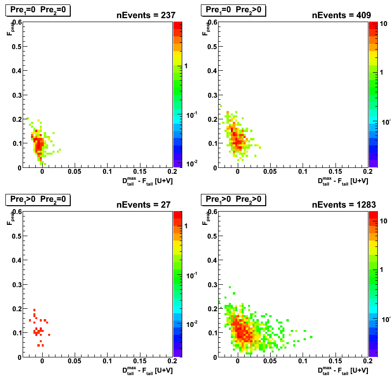
Figure 2: Sided residual for data-driven MC (partonic pt 9-11)

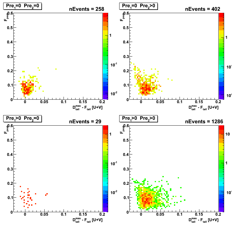
Figure 3: Sided residual for data (pp Longitudinal 2006)

Different analysis cuts vs number of events which passed the cut

N_events : total number of di-jet events found by the jet-finder for gamma in eta region [1,2]
(Geant record is used to get this number)
cos(phi_gamma - phi_jet) < -0.8 : gamma-jet opposite in phi
R_{3x3cluster} > 0.9 : Energy in 3x3 cluster of EEMC tower to the total jet energy.
R_EM^jet < 0.9 : neutral energy fraction cut for on away side jet
N_ch=0 : no charge tracks associated with a gamma candidate
N_bTow = 0 : no barrel towers associated with a gamma candidate (gamma in the endcap)
N_(5-strip clusler)^u > 3 : minimum number of strips in EEMC SMD u-plane cluster around peak
N_(5-strip cluster)^v > 3 : minimum number of strips in EEMC SMD v-plane cluster around peak
gamma-algo fail : my algorithm failed to match tower with SMD uv-intersection, etc...
Tow:SMD match : SMD uv-intersection has a tower which is not in a 3x3 cluser

Figure 4: Number of events which passed various cuts (MC data, partonic pt 9-11)

2008.04.17 Sided residual: Data Driven MC vs raw MC (partonic pt=5-35) vs 2006 data

Ilya Selyuzhenkov April 17, 2008

MC data for different pt weigted according to Michael Betancourt web page:
weight = xSection[ptBin] / xSection[max] / nFiles

Figure 1: Sided residual for raw MC (partonic pt 5-35)
(same plot for partonic pt 9-11)

Figure 2: Sided residual for data-driven MC (partonic pt 5-35)
(same plot for partonic pt 9-11)

Figure 3: Sided residual for data (pp Longitudinal 2006)

Figure 4: Sided residual for data (pp Longitudinal 2006)

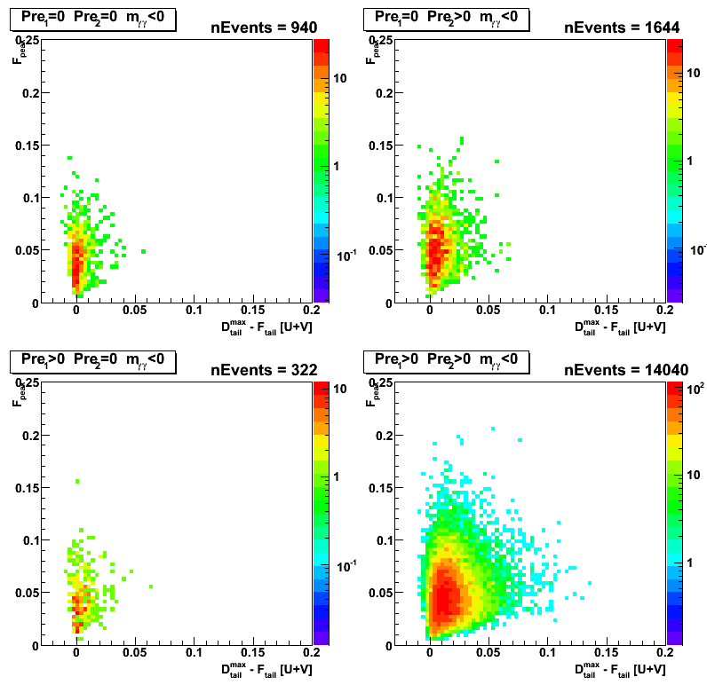
Figure 5: Sided residual for data (pp Longitudinal 2006)

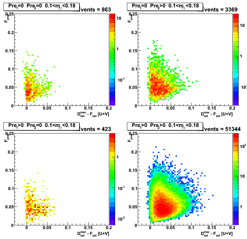
Figure 6: pt(gamma) from geant record vs
pt(gamma) from energy in 3x3 tower cluster and position for uv-intersection wrt vertex
(same on a linear scale)

Figure 7: pt(gamma) from geant record vs
pt(jet) as found by the jet-finder

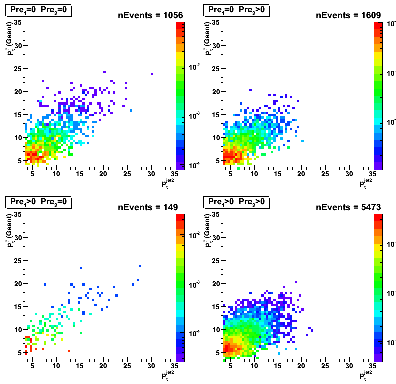
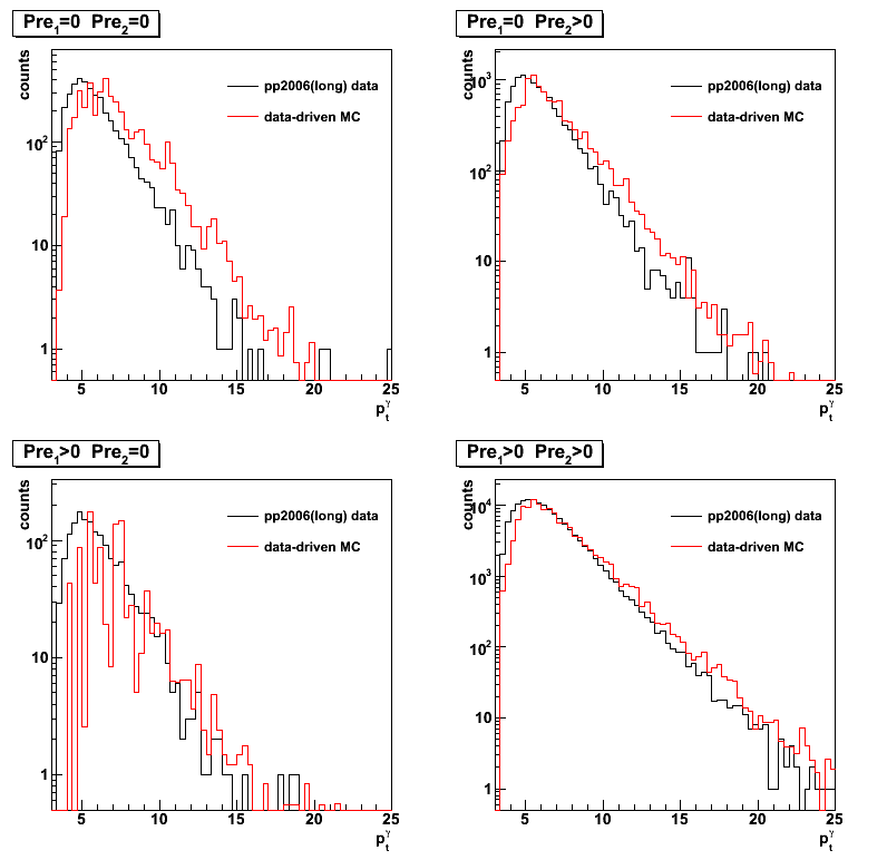
Figure 8: gamma pt distribution:
data-driven MC (red) vs gamma-jet candidates from pp2006 longitudinal run (black).
MC distribution normalized to data at maximum for each preshower condition

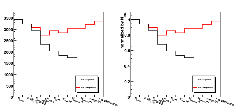
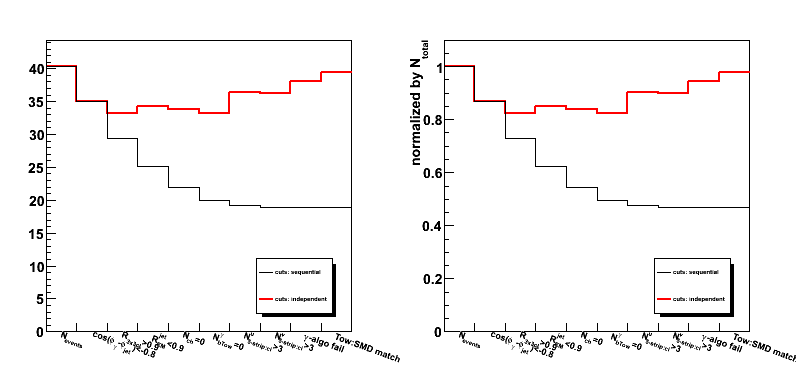
Different analysis cuts vs number of events which passed the cut

N_events : total number of di-jet events found by the jet-finder for gamma in eta region [1,2]
(Geant record is used to get this number)
cos(phi_gamma - phi_jet) < -0.8 : gamma-jet opposite in phi
R_{3x3cluster} > 0.9 : Energy in 3x3 cluster of EEMC tower to the total jet energy.
R_EM^jet < 0.9 : neutral energy fraction cut for on away side jet
N_ch=0 : no charge tracks associated with a gamma candidate
N_bTow = 0 : no barrel towers associated with a gamma candidate (gamma in the endcap)
N_(5-strip clusler)^u > 3 : minimum number of strips in EEMC SMD u-plane cluster around peak
N_(5-strip cluster)^v > 3 : minimum number of strips in EEMC SMD v-plane cluster around peak
gamma-algo fail : my algorithm failed to match tower with SMD uv-intersection, etc...
Tow:SMD match : SMD uv-intersection has a tower which is not in a 3x3 cluser

Figure 9: Number of events which passed various cuts (MC data, partonic pt 5-35)
Red: cuts applied independent
Black: cuts applied sequential from left to right

2008.04.23 Gamma-jet candidates: pp2006 data vs data-driven MC (gamma-jet and bg:jet-jet)

Ilya Selyuzhenkov April 23, 2008

Sided residual: pp2006 data vs data-driven MC (gamma-jet and bg:jet-jet)

MC data for different partonic pt are weigted according to Michael Betancourt web page:
weight = xSection[ptBin] / xSection[max] / nFiles

Figure 1:Sided residual for data-driven gamma-jet MC events (partonic pt 5-35)

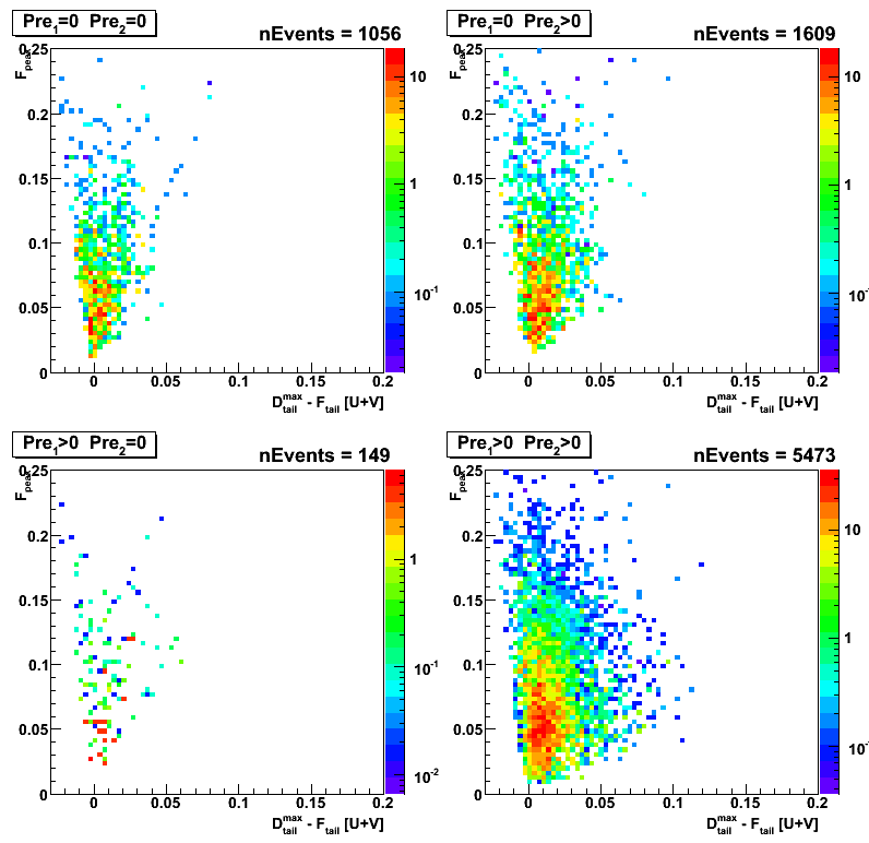
Figure 2:Sided residual for data-driven jet-jet MC events (partonic pt 3-55)

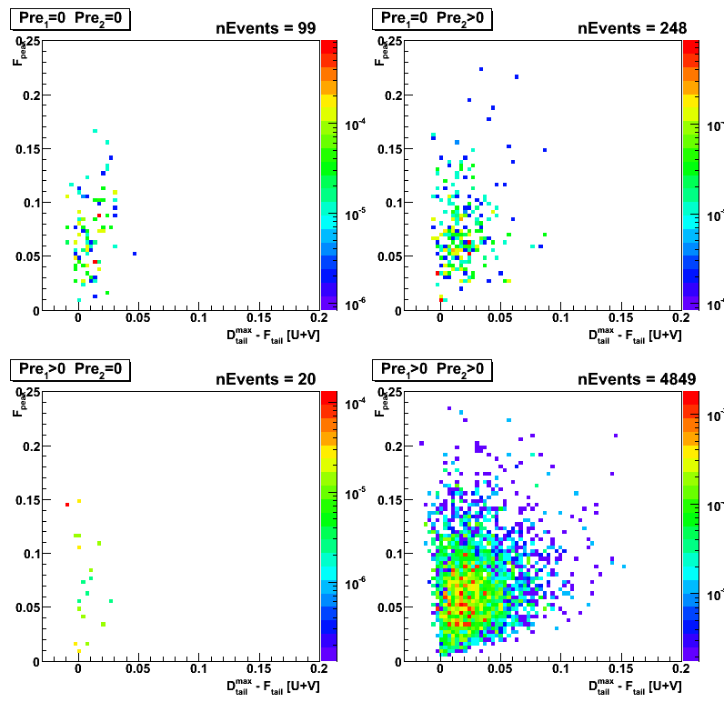
Figure 3:Sided residual for data (pp Longitudinal 2006)

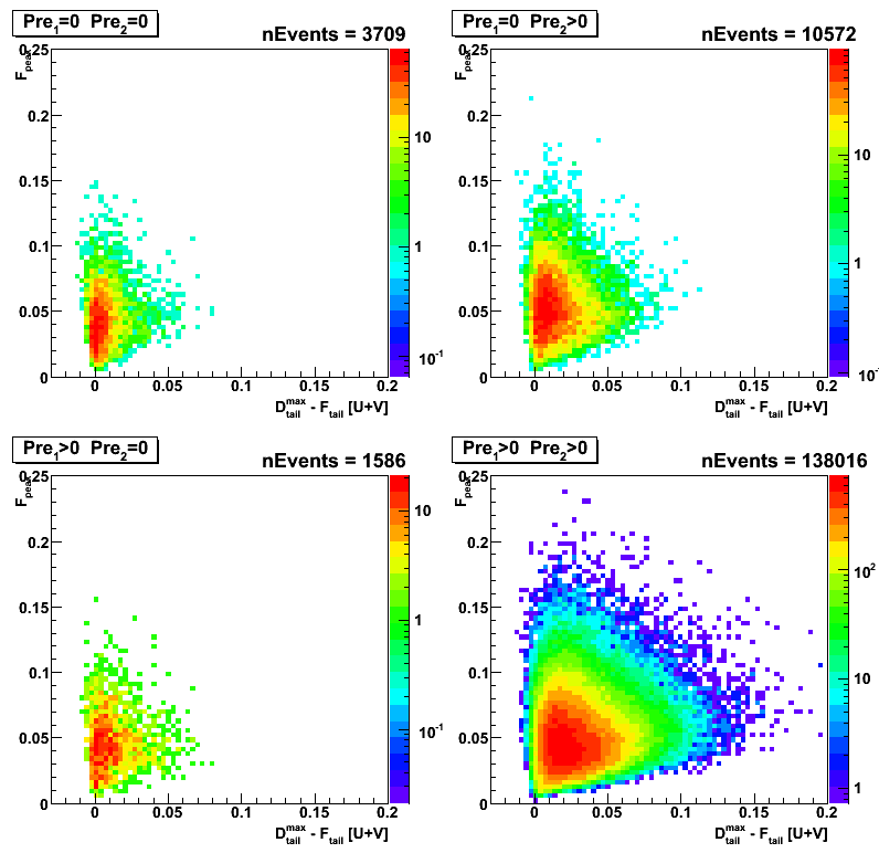
Figure 4:pt(gamma) vs pt(jet) for data-driven gamma-jet MC events (partonic pt 5-35)

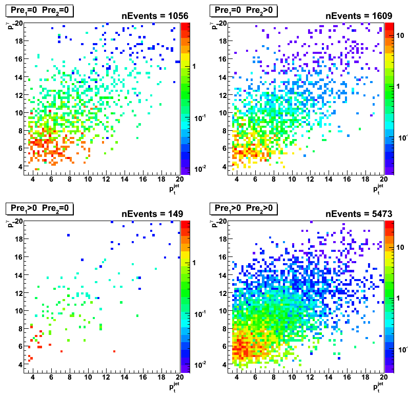
Figure 5:pt(gamma) vs pt(jet) for data-driven jet-jet MC events (partonic pt 3-55)

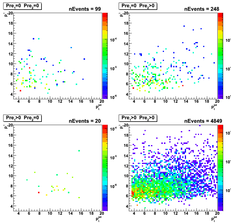
Figure 6:pt(gamma) vs pt(jet) for data (pp Longitudinal 2006)

05 May

May 2008 posts

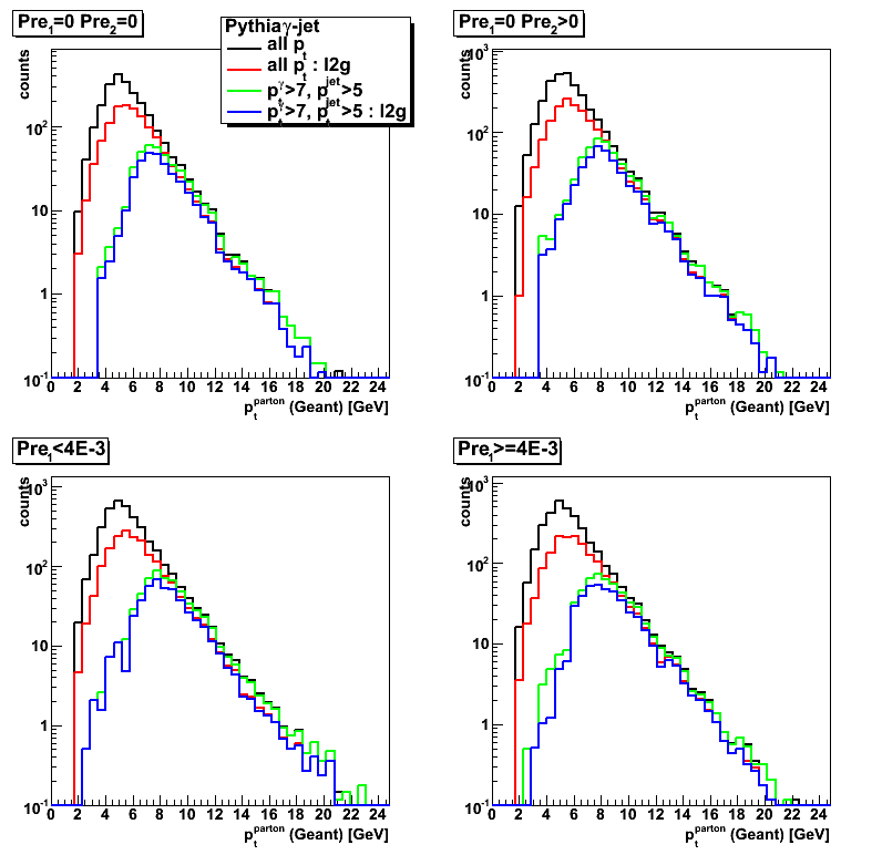
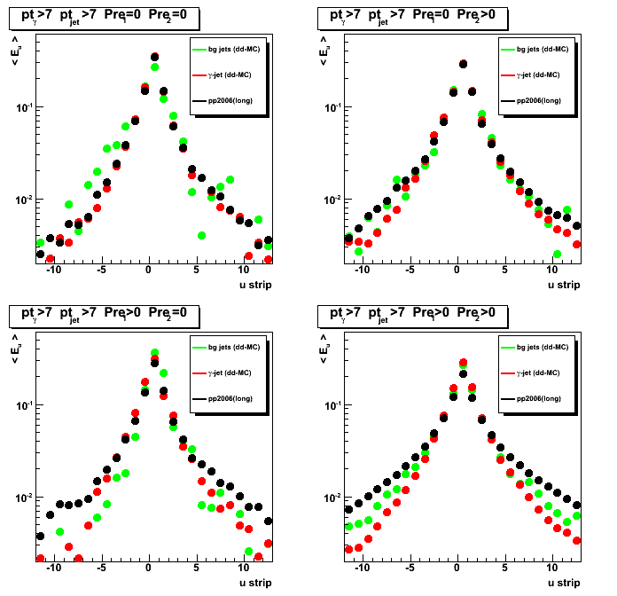
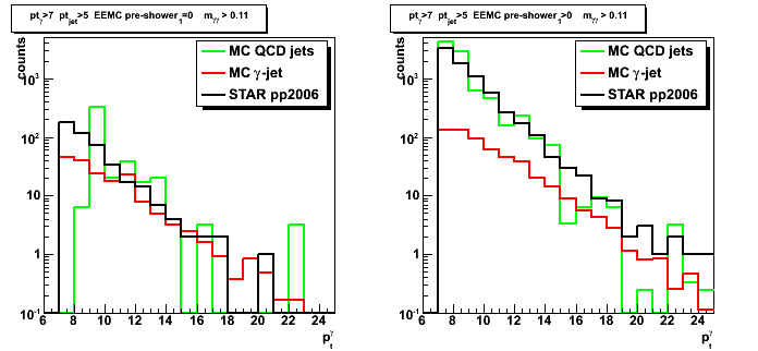
2008.05.05 pt-distributions, sided residual (data vs dd-MC g-jet and bg di-jet)

Ilya Selyuzhenkov May 05, 2008

Data samples:

pp2006(long) - 2006 pp production longitudinal data after applying gamma-jet aisolation cuts
(jet-tree sample: 4.114pb^-1 from Jamie script, 3.164 pb^1 analyses).
gamma-jet - Pythia gamma-jet sample (~170K events). Partonic pt range 5-35 GeV
bg jets - Pythia di-jet sample (~4M events). Partonic pt range 3-65 GeV

Figure 1:pt distribution. MC data are scaled to the same luminosity as data
(Normalization factor: Luminosity * sigma / N_events).

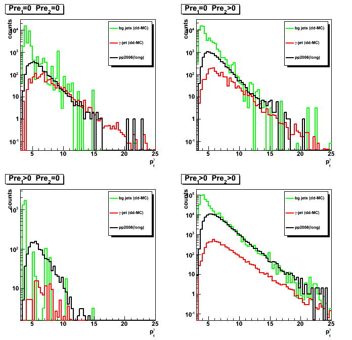
Figure 2:Integrated gamma yield vs pt.
For each pt bin yield is defined as the integral from this pt up to the maximum available pt.
MC data are scaled to the same luminosity as data.

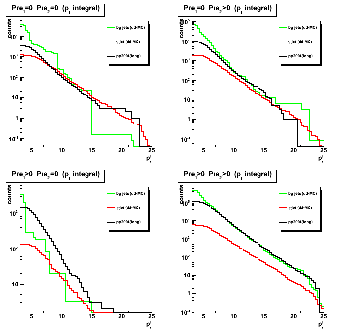
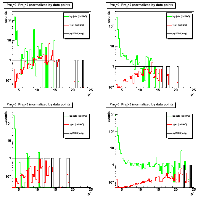
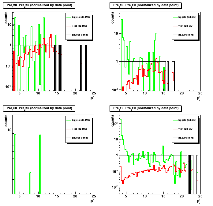
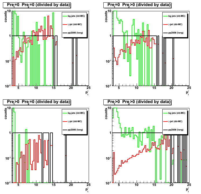
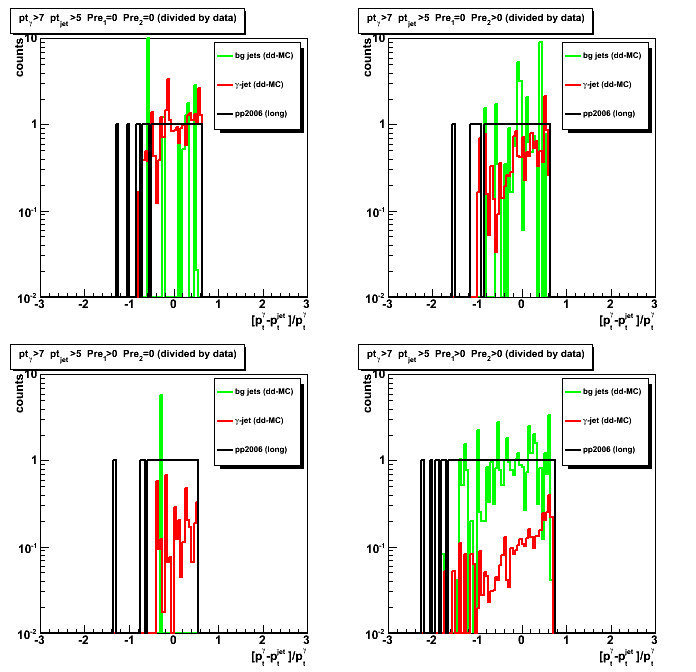
Figure 3:Signal to background ratio (all results divided by the data)

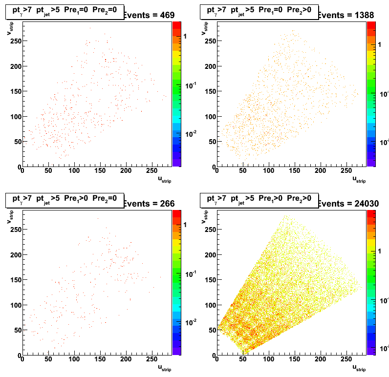
Sided residual: pp2006 data vs data-driven MC (gamma-jet and bg:jet-jet)

You can find sided residual 2-D plots here

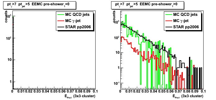
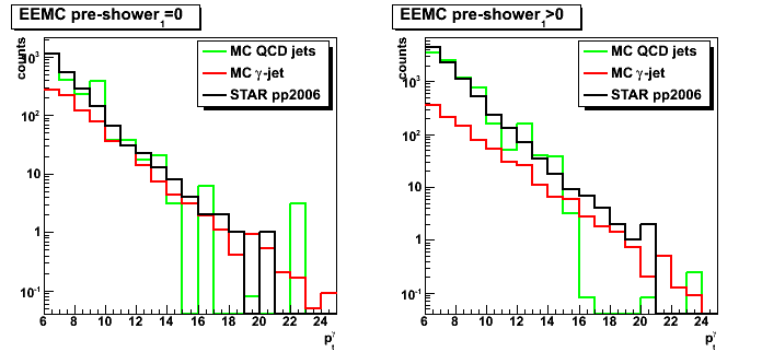
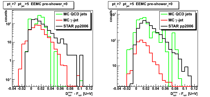
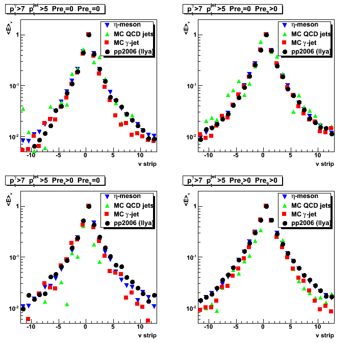
Figure 4:Maximum sided residual for pt_gamma>7GeV; pt_jet>7GeV

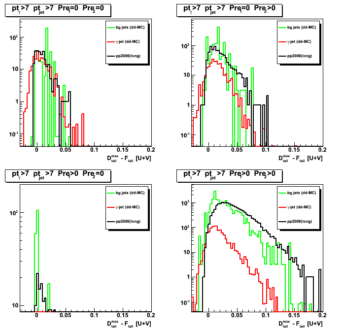
Figure 5:Fitted peak for pt_gamma>7GeV; pt_jet>7GeV

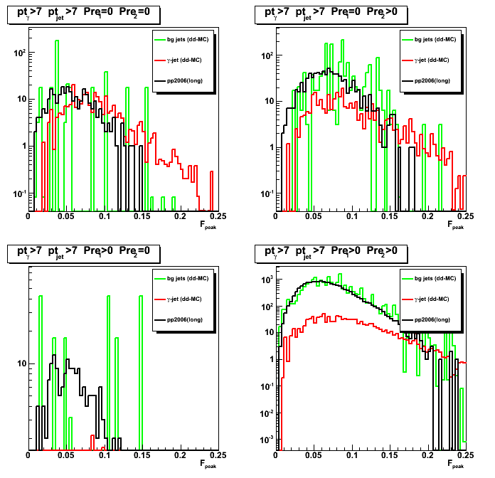
Figure 6:Max data tail for pt_gamma>7GeV; pt_jet>7GeV

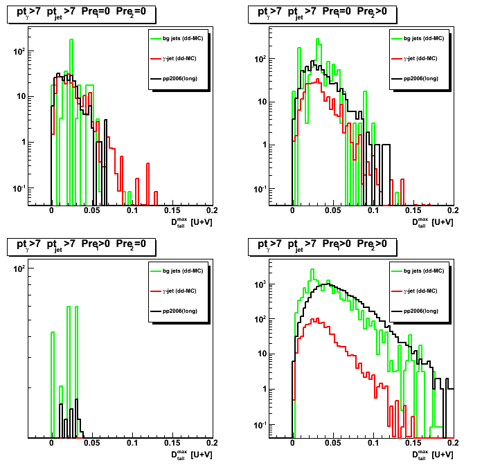
Figure 7:Max minus min data tails for pt_gamma>7GeV; pt_jet>7GeV

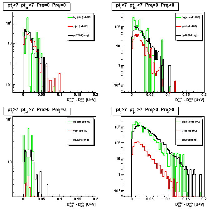
Figure 8:Shower shapes pt_gamma>7GeV; pt_jet>7GeV

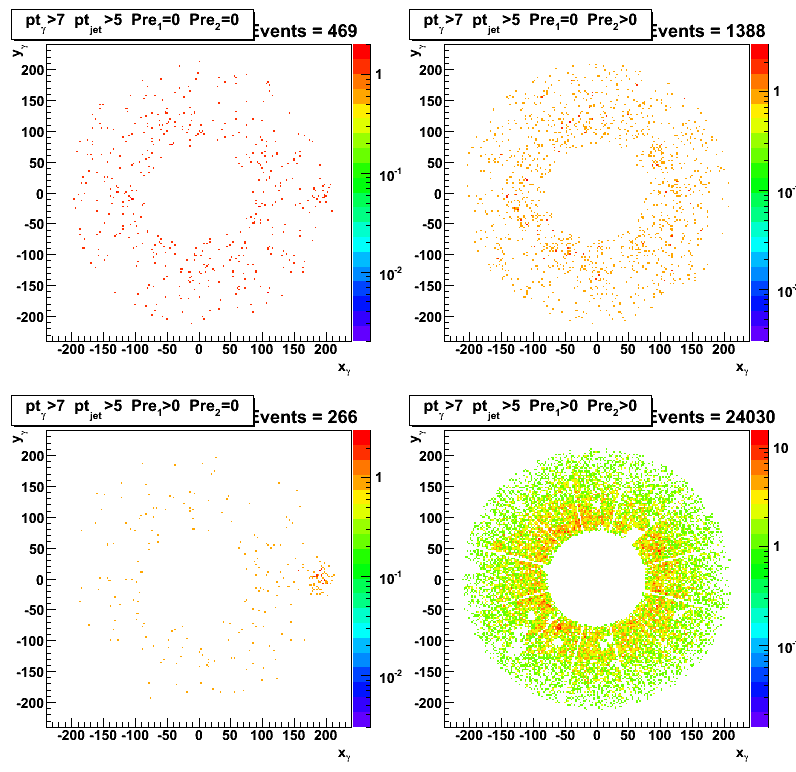
2008.05.08 y:x EEMC position for gamma-jet candidates

Ilya Selyuzhenkov May 08, 2008

y:x EEMC position for gamma-jet candidates

Figure 1:y:x EEMC position for gamma-jet candidates:
Pythia gamma-jet sample (~170K events). Partonic pt range 5-35 GeV.

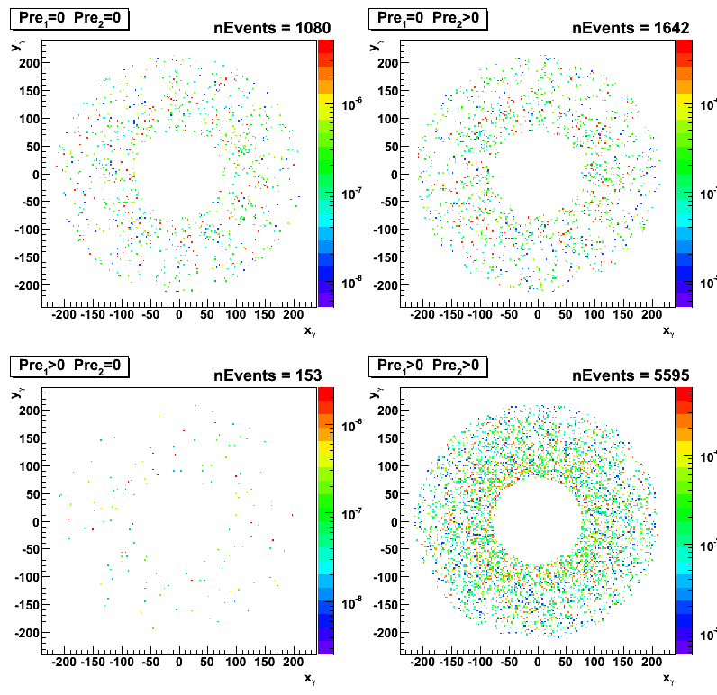
Figure 2:y:x EEMC position for gamma-jet candidates:
Pythia QCD bg sample (~4M events). Partonic pt range 3-65 GeV.

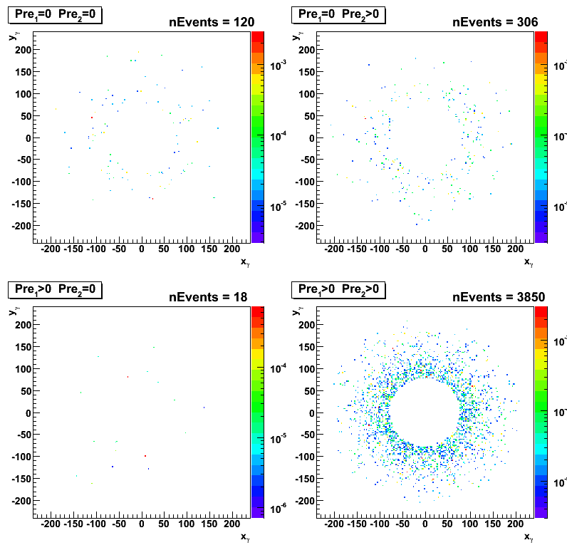
Figure 3:y:x EEMC position for gamma-jet candidates:
pp2006 (long) data [eemc-http-mb-l2gamma:137641 trigger]

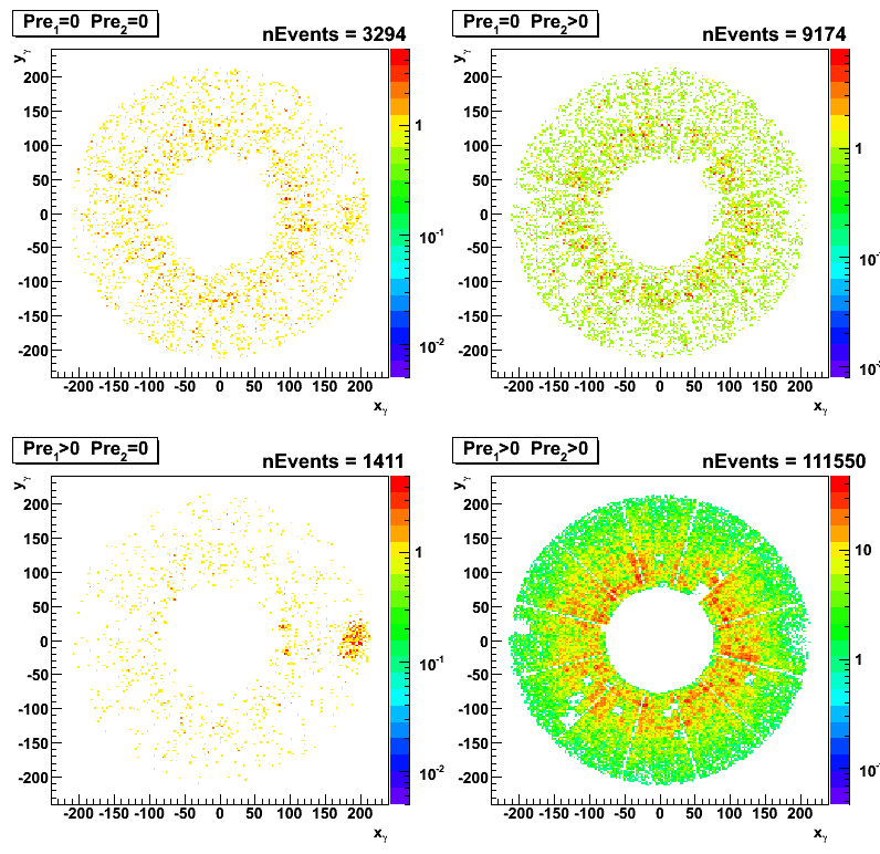
Figure 3b:y:x EEMC position for gamma-jet candidates:
pp2006 (long) data [eemc-http-mb-l2gamma:137641 trigger]
pt cut of 7 GeV for gamma and 5GeV for the away side jet has been applied.

high u vs. v strip for gamma-jet candidates

Figure 4:High v-strip vs high u-strip.
Pythia gamma-jet sample (~170K events). Partonic pt range 5-35 GeV.

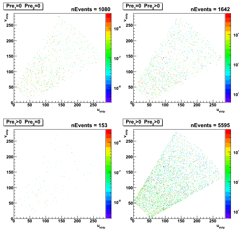
Figure 5:High v-strip vs high u-strip:
Pythia QCD bg sample (~4M events). Partonic pt range 3-65 GeV.

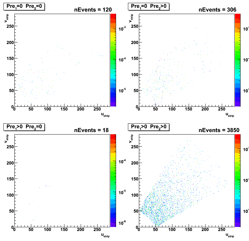
Figure 6:High v-strip vs high u-strip:
pp2006 (long) data [eemc-http-mb-l2gamma:137641 trigger]

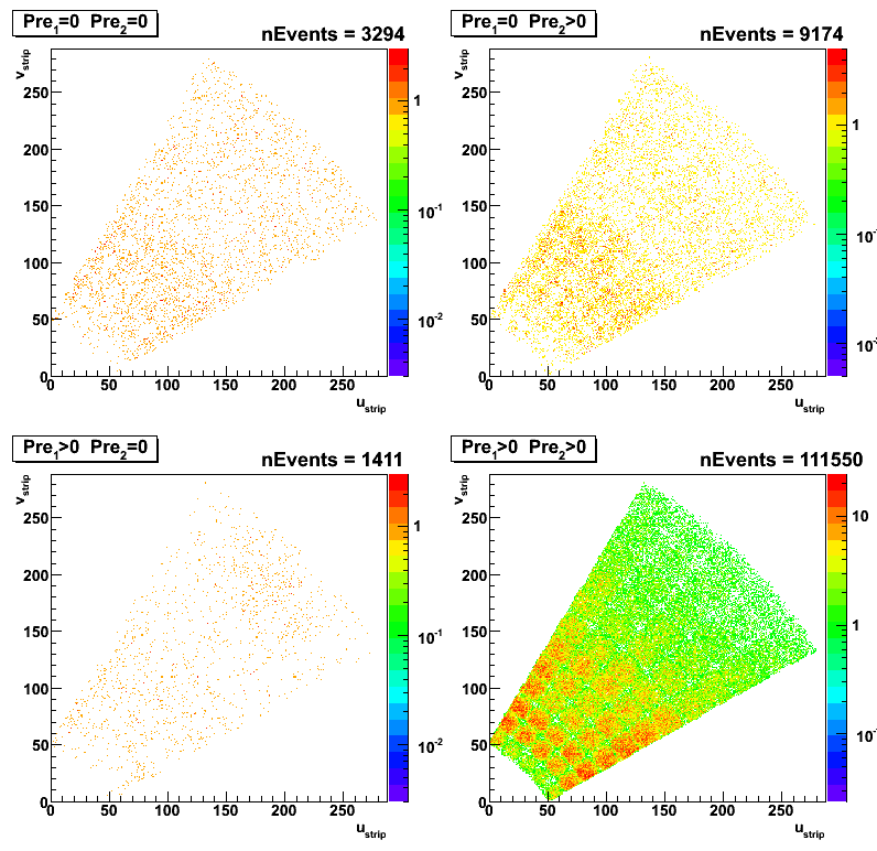
Figure 6b:High v-strip vs high u-strip:
pp2006 (long) data [eemc-http-mb-l2gamma:137641 trigger]
pt cut of 7 GeV for gamma and 5GeV for the away side jet has been applied.

2008.05.09 Gamma-jet candidates pt-distributions and TPC tracking

Ilya Selyuzhenkov May 09, 2008

Detector eta cut study (1< eta < 1.4):

For a three data samples (pp2006 [long], MC gamma-jet, and MC QCD background events)
the EEMC detector eta cut of 1< eta < 1.4 has been applied.
Although a poor statistics available for MC background QCD sample,
the signal to background ratio (red to green line ratio)
getting closer to 1:3 (expected signal to background ratio from Les study).
Distributions withoud EEMC detector eta cut.
y:x position within EEMC detector for gamma-jet candidates.

Figure 1:Gamma pt distribution. MC data are scaled to the same luminosity as data
(Normalization factor: Luminosity * sigma / N_events).

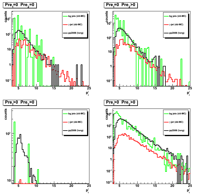
Figure 2:Gamma yield vs pt. MC data are scaled to the same luminosity as data.

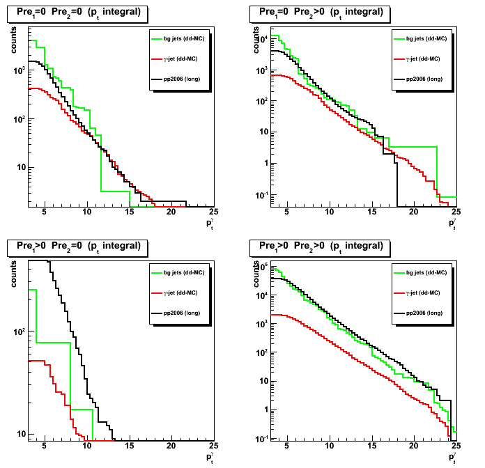
Figure 3:Signal to background ratio (MC results are normalized to the data)

2008.05.14 Gamma-cluster to jet energy ratio and away side jet pt matching

Ilya Selyuzhenkov May 14, 2008

Gamma-cluster to jet1 energy ratio

Correlation between gamma-candidate 3x3 cluster energy ratio (R_cluster) and
number of EEMC towers in a jet1 can be found here (Fig. 4).
Gamma pt distribution, yield and signal to background ratio plots
for a cut of R_cluster >0.9 can be found here (Figs. 1-3).
Gamma pt distribution, yield and signal to background ratio plots
for a cut of R_cluster >0.99 are shown below in Figs. 1-3.
One can see that by going from R_cluster>0.9 to R_cluster>0.99
improves signal to background ratio from ~ 1:10 to ~ 1:5 for gamma pt>10 GeV

Figure 1:Gamma pt distribution for R_cluster >0.99.
MC results scaled to the same luminosity as data
(Normalization factor: Luminosity * sigma / N_events).

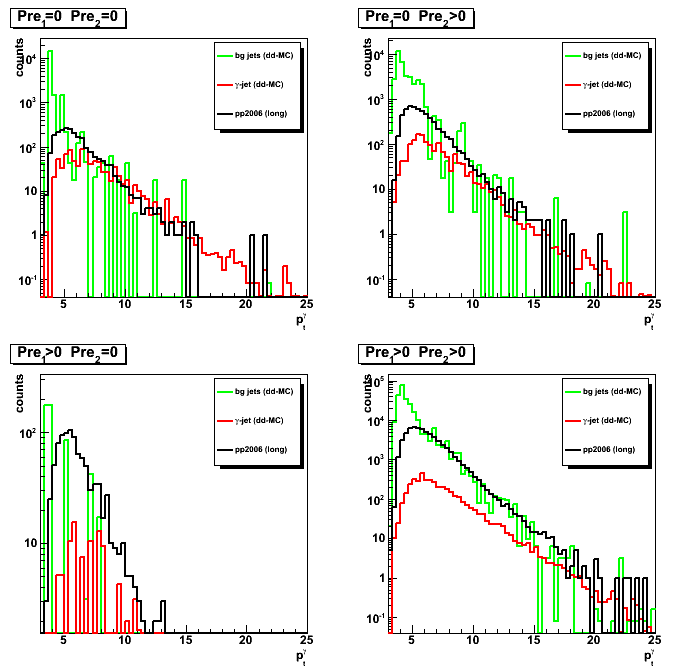
Figure 2:Integrated gamma yield vs pt for R_cluster >0.99
For each pt bin yield is defined as the integral from this pt up to the maximum available pt.
MC results scaled to the same luminosity as data.

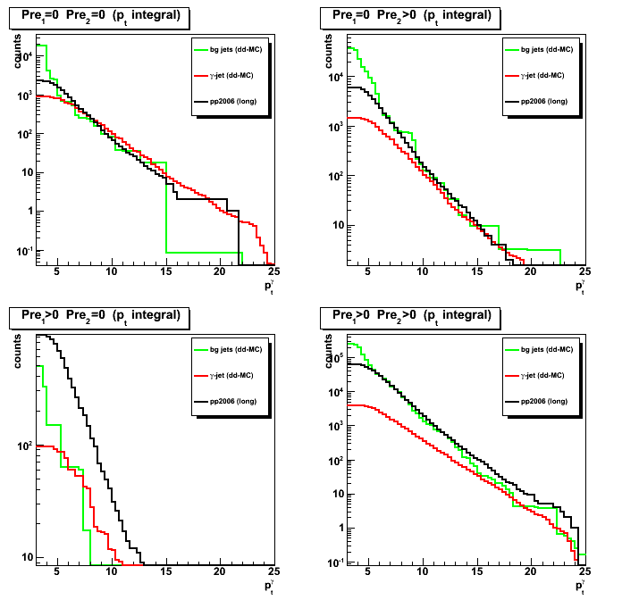
Figure 3:Signal to background ratio for R_cluster >0.99 (all results divided by the data)
Compare this figure with that for R_cluster>0.9 (Fig. 3 at this link)

Gamma and the away side jet pt matching

Figure 4: pt asymmetry between gamma and the away side jet (R_cluster >0.9)
for a three data samples (pp2006[long] data, gamma-jet MC, QCD jets background).
pt cut of 7 GeV for both gamma and jet has been applied.

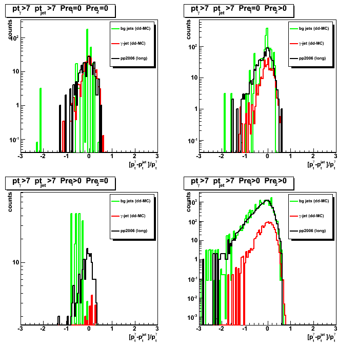
Figure 5: signal to background ratio (R_cluster >0.9)
as a function of pt asymmetry between gamma and the away side jet
pt cut of 7 GeV for both gamma and jet has been applied.

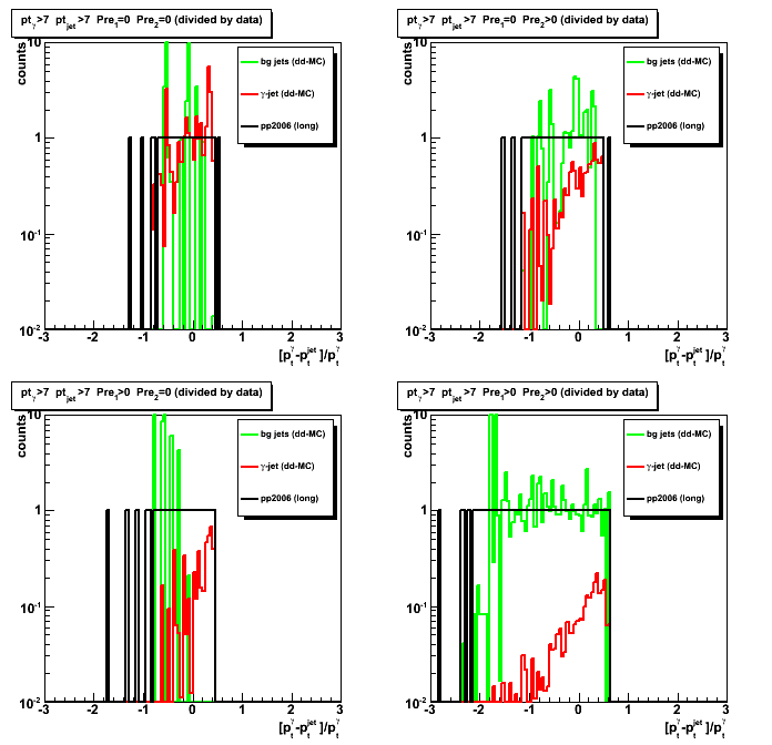
Figure 6: pt asymmetry between gamma and the away side jet (R_cluster >0.99)
for a three data samples (pp2006[long] data, gamma-jet MC, QCD jets background).
pt cut of 7 GeV for both gamma and jet has been applied.

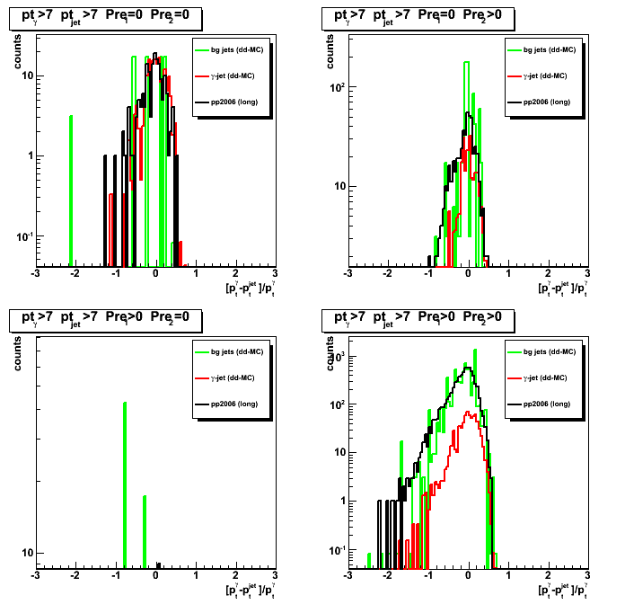
Figure 7: signal to background ratio
as a functio of pt asymmetry between gamma and the away side jet (R_cluster >0.99)
pt cut of 7 GeV for both gamma and jet has been applied.

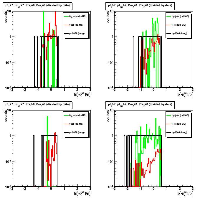
Figure 8: pt asymmetry between gamma and the away side jet (R_cluster >0.99)
for a three data samples (pp2006[long] data, gamma-jet MC, QCD jets background).
pt cut of 7 GeV for gamma and 5GeV for the away side jet has been applied.

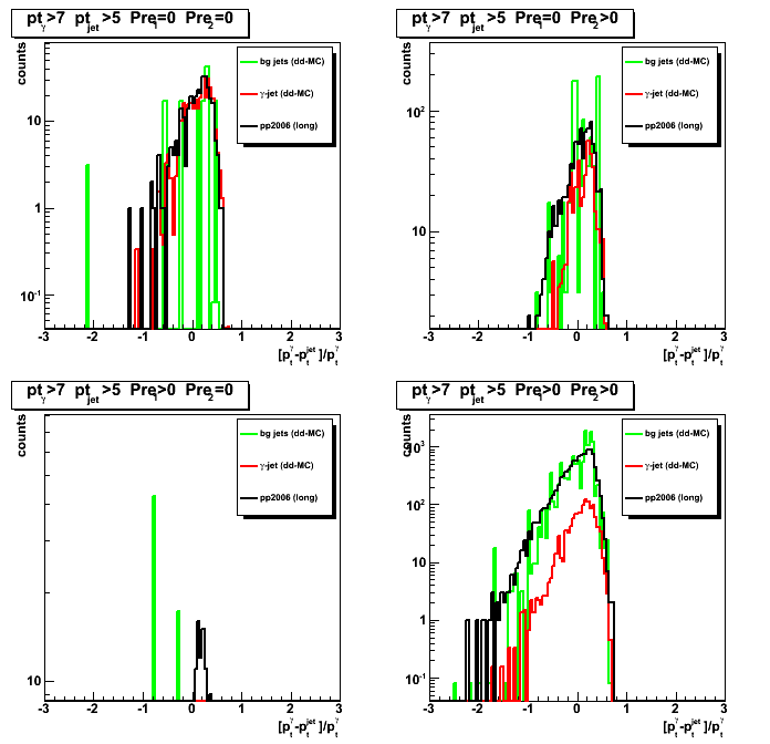
Figure 9: signal to background ratio
as a function of pt asymmetry between gamma and the away side jet (R_cluster >0.99)
pt cut of 7 GeV for gamma and 5GeV for the away side jet has been applied.

2008.05.15 Vertex z distribution for pp2006 data, MC gamma-jet and QCD jets events

Ilya Selyuzhenkov May 15, 2008

Figure 1:Vertex z distribution for pp2006 (long) data [eemc-http-mb-l2gamma:137641 trigger]
Note: In the upper right plot (pre1=0, pre2>0) one can see
a hole in the acceptance in the range bweeeen z_vertex -10 to 30 cm (probably due to SVT construction)

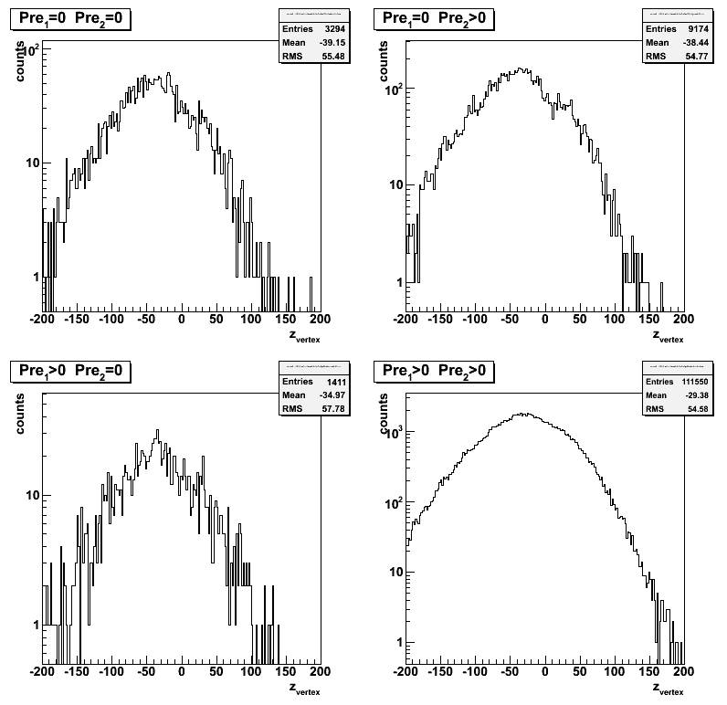
Figure 1b:Vertex z distribution for pp2006 (same as Fig. 1, but on a linear scale)

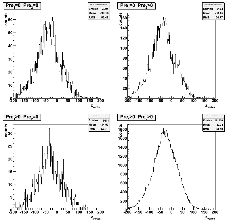
Figure 2:Vertex z distribution for three different data samples
MC results scaled to the same luminosity as data

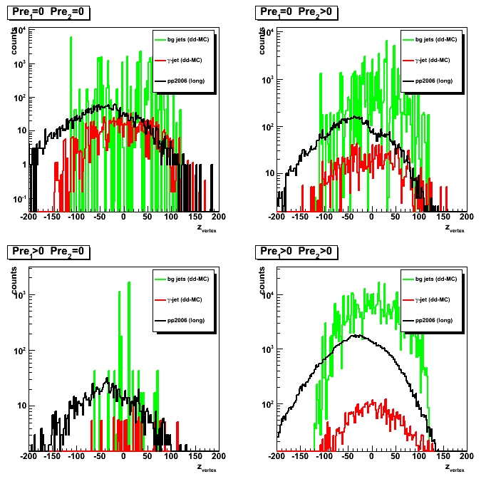
Figure 3:Vertex z distribution for three different data samples
pt cut of 7 GeV for gamma and 5GeV for the away side jet has been applied.

2008.05.20 Shower shapes sorted by pre-shower, z-vertex and gamma's eta, phi, pt

Ilya Selyuzhenkov May 20, 2008

Gamma-jet algorithm and isolation cuts:

Selecting only di-jet events identified by the STAR jet finder algorithm,
with jets pointing opposite in azimuth:
cos(phi_jet1 - phi_jet2) < -0.8
Select jet1 with a maximum neutral energy fraction (R_EM1).
This is our gamma candidate, for which we further require:
- No charge tracks associated with jet1 (default jet radius is 0.7):
  nChargeTracks_jet1 = 0
  Note, that this charge track veto only works
  in the EEMC region where we do have TPC tracking
- No barrel towers associated with jet1 (pure EEMC jet):
  nBarrelTowers_jet1 = 0
- Ratio of the energy in the 3x3 EEMC high tower cluster
  to the total jet energy to be:
  R_cluster>0.99 (previous, softer, cut was 0.9)
For the second jet2 (away side jet) we require:
- That jet2 has at least ~10% of hadronic energy:
  R_EM2<0.9
Additional gamma candidate QA requirements:
- Matching between EEMC SMD uv-strip cluster with a 3x3 cluster of EEMC towers.
  (in addition reject events for which we can not idetify uv-strip intersection)
- Minimum number of strips in 5-strip EEMC SMD uv-plane clusters to be greater that 3.

Data sample:

pp2006(long) - 2006 pp production longitudinal data after applying gamma-jet isolation cuts
(note the new R_cluster>0.99 cut)

Shower shapes sorted by pre-shower, z-vertex and gamma's eta, phi, pt

Note, that all shapes are normalized at peak to unity

Figure 1:Shower shapes for different detector eta bins

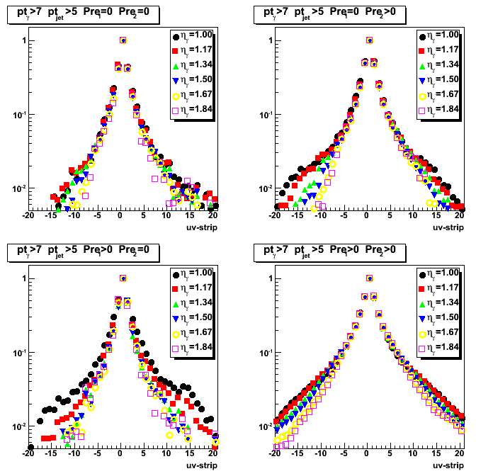
Figure 2:Shower shapes for different detector phi bins

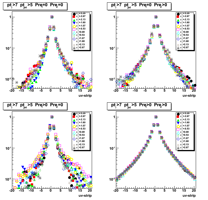
Figure 3:Shower shapes for different gamma pt bins

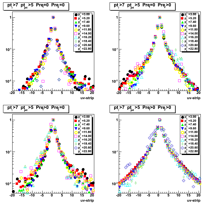
Figure 4:Shower shapes for different z-vertex bins

2008.05.21 EEMC SMD data-driven library: some eta-meson QA plots

Ilya Selyuzhenkov May 21, 2008

EEMC SMD data-driven library: some eta-meson QA plots

Data sample:

Subset of 441 eta-meson candidates from Will's analysis.
additional QA info (detector eta, pre1, pre2, etc)
has been added to pi0-tree reader script:
/star/institutions/iucf/wwjacobs/newEtas_fromPi0finder/ReadEtaTree.C
pi0 trees from this RCF directory has been used to regenerate etas NTuple:
/star/institutions/iucf/wwjacobs/newEtas_fromPi0finder/out_23/

Some observations:

eta-meson purity within the invariant mass region [0.5, 0.65] is about 72%
Most of the eta-candidates has detector pseudorapidity less or about 1.4,
what may limits applicability of data-driven shower shapes
derived from these candidates for higher pseudo-rapidity region,
where we have most of the background for the gamma-jet
analysis due to lack of TPC tracking
z-vertex distribution is very asymmetric, and peaked around -50cm.
Only a few candidates has a positive z-vertex values.

Figure 1: Eta-meson invariant mass with signal and background fits and ratio (upper left).
Pseudorapidity [detector and wrt vertex] distributions (right top and bottom plots),
vertex z distributions (bottom left)

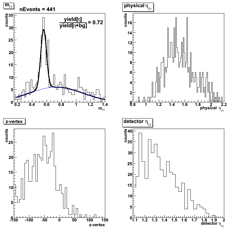
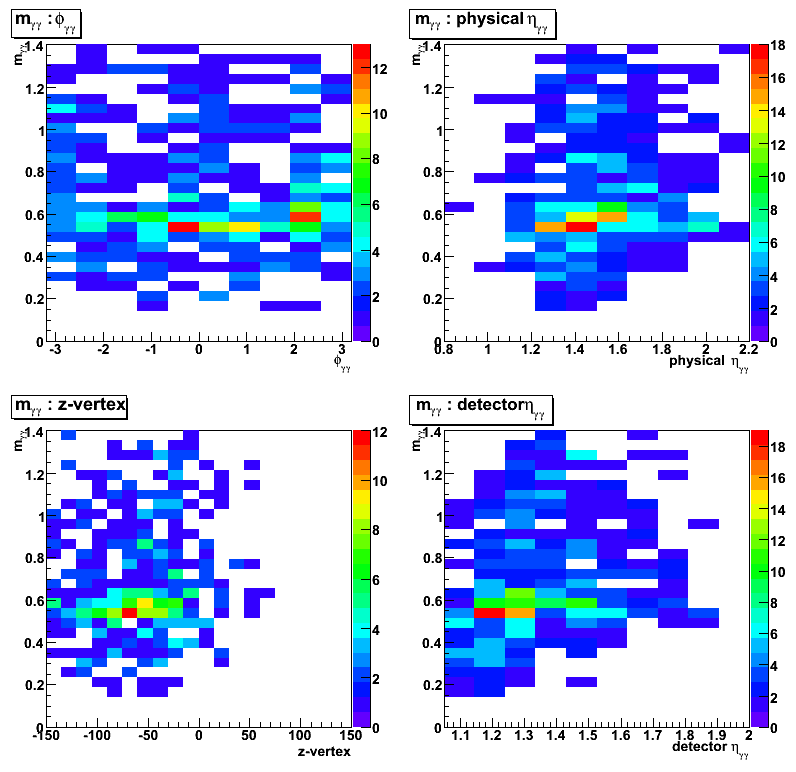
Figure 2:2D plots for the eta-meson invariant mass vs
azimuthal angle (upper left), pseudorapidity (upper right),
z-vertex (bottom right), and detector pseudorapidity (bottom right)

2008.05.27 Shower shapes: pp2006 data, MC gamma-jet and QCD jets, gammas from eta

Ilya Selyuzhenkov May 27, 2008

Shower shapes and triple Gaussian fits for gammas from eta-meson

Figure 1: Shower shapes and triple Gaussian fits for photons from eta-meson
sorted by different conditions of EEMC 1st and 2nd pre-shower layers.
Note: All shapes have been normalized at peak to unity

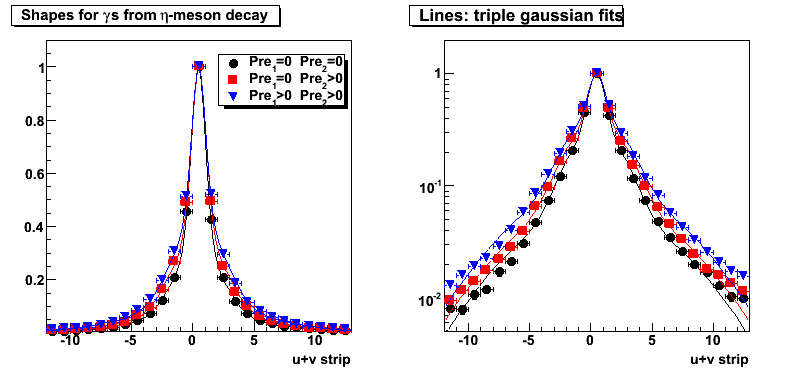
Triple Gaussian fit parameters:
Pre1=0 Pre2=0
0.669864*exp(-0.5*sq((x-0.46016)/0.574864))+0.272997*exp(-0.5*sq((x-0.46016)/-1.84608))+0.0585682*exp(-0.5*sq((x-0.46016)/5.49802))
Pre1=0 Pre2>0
0.0694729*exp(-0.5*sq((x-0.493468)/5.65413))+0.615724*exp(-0.5*sq((x-0.493468)/0.590723))+0.314777*exp(-0.5*sq((x-0.493468)/2.00192))
Pre1>0 Pre2>0
0.0955638*exp(-0.5*sq((x-0.481197)/5.59675))+0.558661*exp(-0.5*sq((x-0.481197)/0.567596))+0.345896*exp(-0.5*sq((x-0.481197)/1.9914))

Shower shapes: pp2006, MC gamma-jet and QCD jets, gammas from eta

Shower shapes comparison between different data sets:

gammas from eta-meson decay. Obtained from Will's eta-meson analysis
pp2006 - STAR 2006 pp longitudinal data (~ 3.164 pb^1) after applying gamma-jet isolation cuts.
gamma-jet - data-driven Pythia gamma-jet sample (~170K events). Partonic pt range 5-35 GeV.
QCD jets - data-driven Pythia QCD jets sample (~4M events). Partonic pt range 3-65 GeV.

Some observations:

Shapes for gammas from eta-meson decay
are in a good agreement with those from MC gamma-jet sample
(compare red squares with blue triangle in Fig. 2 and 3).

MC gamma-jet shapes obtained by running a full gamma-jet reconstruction algorithm,
and this agreement indicates that we are able to reconstruct gamma shapes
which we put in with data-driven shower shape library.
MC gamma-jet shapes match pp2006 data shapes
for pre1=0 condition, where we expect to be very efficient in background rejection
(compare red squares with black circles in upper plots of Fig. 2 and 3).

This indicates that we are able to reproduce EEMC SMD of direct photons with data-driven Monte-Carlo.
There is no match between Monte-Carlo QCD background jets and pp2006 data
for the case when both pre-shower layer fired (pre1>0 and pre2>0).
(compare green triangles with black circes in bottom right plots of Fig.2 and 3).
This is the region where we know background dominates our gamma-jet candidates.

This shows that we still do not reproduce SMD response for our background events
in our data-driven Monte-Carlo simulations
(note, that in Monte-Carlo we replace SMD response with real shapes for all background photons
the same way we do it for direct gammas).

Figure 2: Shower shapes comparison between different data sets.
Shapes for gamma-jet candidates obtained with the same gamma-jet reconstruction algorithm
for three different data samples (pp2006, gamma-jet and QCD jets MC).
pt cuts of 7GeV for the gamma and of 5 GeV for the away side jet have been applied.

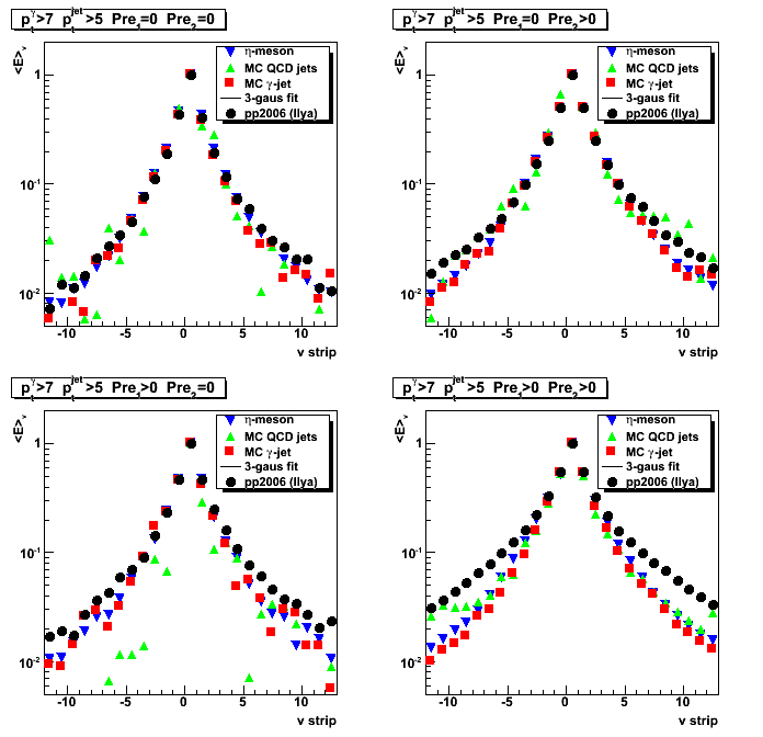
Figure 3:Same as Fig. 2, but with no cuts on gamma and jet pt.
All shapes are similar to those in Fig. 2 with an additional pt cuts.
Note, that blue triangles are the same as in Fig. 2.

2008.05.30 Eta, phi, and pt distributions for gamma and jet from MC and pp2006 data

Ilya Selyuzhenkov May 30, 2008

Three data sets:

pp2006 - STAR 2006 pp longitudinal data (~ 3.164 pb^1) after applying gamma-jet isolation cuts.
gamma-jet - data-driven Pythia gamma-jet sample (~170K events). Partonic pt range 5-35 GeV.
QCD jets - data-driven Pythia QCD jets sample (~4M events). Partonic pt range 3-65 GeV.

Figure 1: Gamma eta distribution.
pt cuts of 7GeV for the gamma and of 5 GeV for the away side jet have been applied.

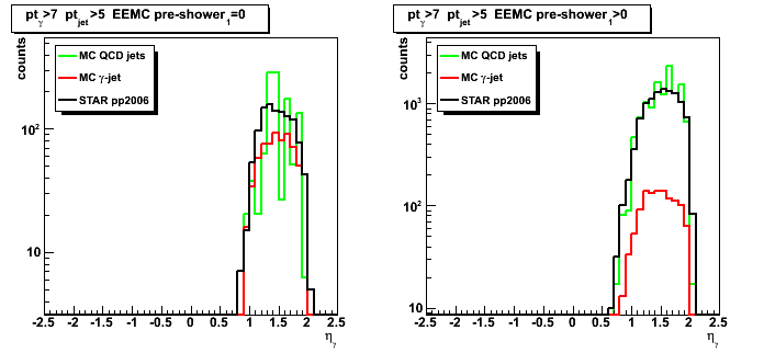
Figure 2: Gamma pt distribution.
pt cuts of 7GeV for the gamma and of 5 GeV for the away side jet have been applied.

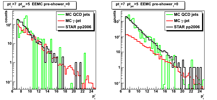
Figure 3: Gamma phi distribution.
pt cuts of 7GeV for the gamma and of 5 GeV for the away side jet have been applied.

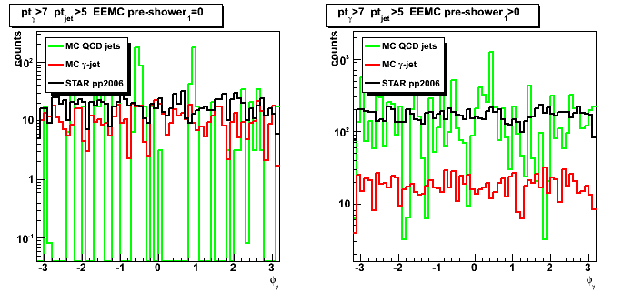
Figure 4: Away side jet eta distribution.
pt cuts of 7GeV for the gamma and of 5 GeV for the away side jet have been applied.

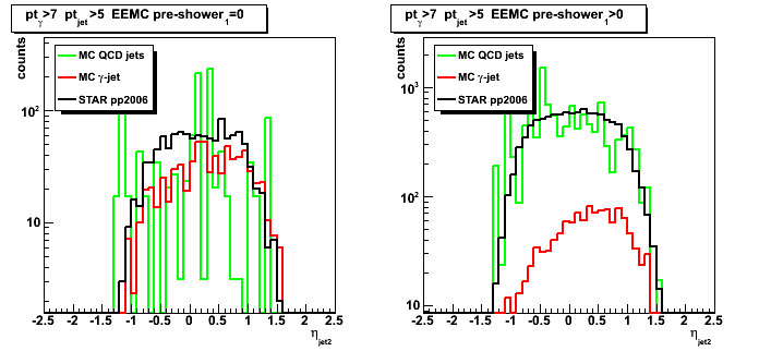
Figure 5: Away side jet pt distribution.
pt cuts of 7GeV for the gamma and of 5 GeV for the away side jet have been applied.

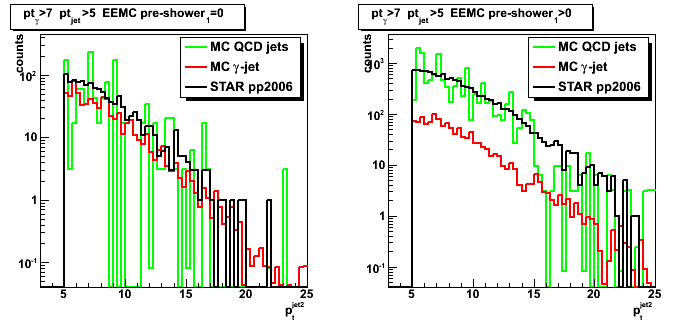
Figure 6: Gamma-jet delta pt distribution.
pt cuts of 7GeV for the gamma and of 5 GeV for the away side jet have been applied.

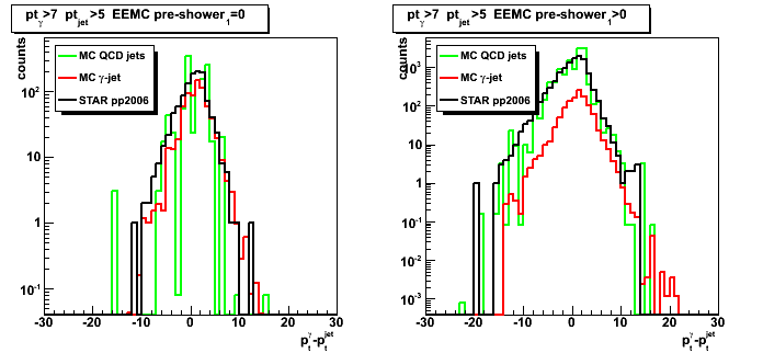
Figure 7: Gamma-jet delta eta distribution.
pt cuts of 7GeV for the gamma and of 5 GeV for the away side jet have been applied.

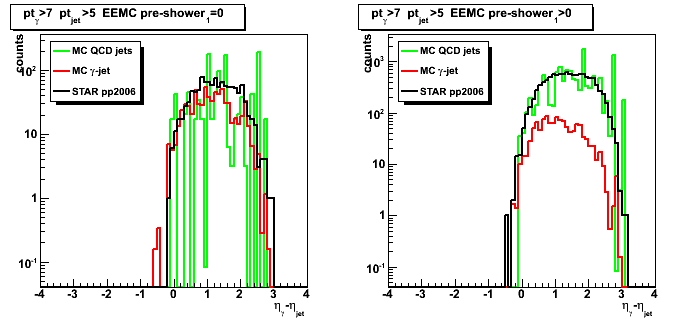
Figure 8: Gamma-jet delta phi distribution.
pt cuts of 7GeV for the gamma and of 5 GeV for the away side jet have been applied.

06 Jun

June 2008 posts

2008.06.04 Gamma cluster energy in various EEMC layers: data vs MC

Ilya Selyuzhenkov June 04, 2008

Gamma cluster energy in various EEMC layers: data vs MC

Three data sets:

pp2006 - STAR 2006 pp longitudinal data (~ 3.164 pb^1) after applying gamma-jet isolation cuts.
gamma-jet - data-driven Pythia gamma-jet sample (~170K events). Partonic pt range 5-35 GeV.
QCD jets - data-driven Pythia QCD jets sample (~4M events). Partonic pt range 3-65 GeV.

Figure 1: Gamma candidate EEMC pre-shower 1 energy (3x3 cluster).
pt cuts of 7GeV for the gamma and of 5 GeV for the away side jet have been applied.

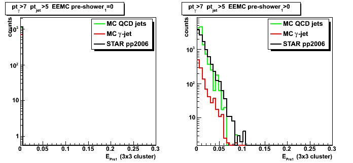
Figure 2: Gamma candidate EEMC pre-shower 2 energy (3x3 cluster).
pt cuts of 7GeV for the gamma and of 5 GeV for the away side jet have been applied.

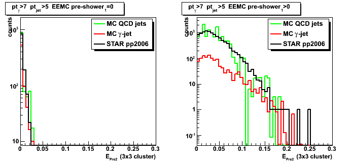
Figure 3: Gamma candidate EEMC tower energy (3x3 cluster).
pt cuts of 7GeV for the gamma and of 5 GeV for the away side jet have been applied.

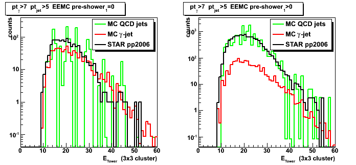
Figure 4: Gamma candidate EEMC post-shower energy (3x3 cluster).
pt cuts of 7GeV for the gamma and of 5 GeV for the away side jet have been applied.

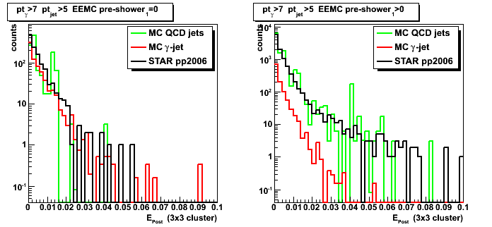
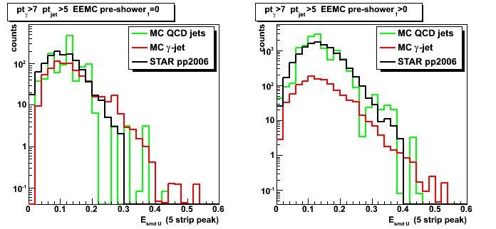
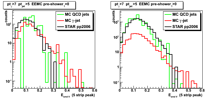
Figure 5: Gamma candidate EEMC SMD u-plane energy [5-strip cluster] (Figure for v-plane)
pt cuts of 7GeV for the gamma and of 5 GeV for the away side jet have been applied.

Difference between total and gamma candidate cluster energy for various EEMC layers

Figure 6: Total minus gamma candidate (3x3 cluster) energy in EEMC pre-shower 1 layer
pt cuts of 7GeV for the gamma and of 5 GeV for the away side jet have been applied.

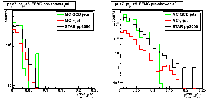
Figure 7: Total minus gamma candidate (3x3 cluster) energy in EEMC pre-shower 2 layer
pt cuts of 7GeV for the gamma and of 5 GeV for the away side jet have been applied.

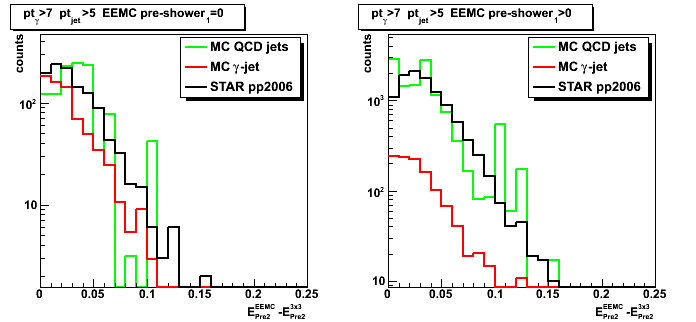
Figure 8: Total minus gamma candidate (3x3 cluster) energy in EEMC tower
pt cuts of 7GeV for the gamma and of 5 GeV for the away side jet have been applied.

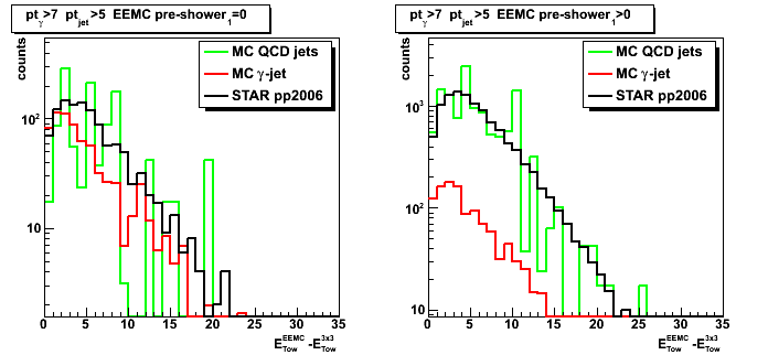
Figure 9: Total minus gamma candidate (3x3 cluster) energy in EEMC post-shower layer
pt cuts of 7GeV for the gamma and of 5 GeV for the away side jet have been applied.

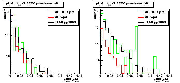
Figure 10: Total (sector) energy minus gamma candidate (5-strip cluster) energy in EEMC SMD[u-v] layer
pt cuts of 7GeV for the gamma and of 5 GeV for the away side jet have been applied.

2008.06.09 STAR White paper plots (pt distribution: R_cluster 0.99 and 0.9 cuts)

Ilya Selyuzhenkov June 09, 2008

Gamma pt distribution: data vs MC (R_cluster 0.99 and 0.9 cuts)

Three data sets:

pp2006 - STAR 2006 pp longitudinal data (~ 3.164 pb^1) after applying gamma-jet isolation cuts.
gamma-jet - data-driven Pythia gamma-jet sample (~170K events). Partonic pt range 5-35 GeV.
QCD jets - data-driven Pythia QCD jets sample (~4M events). Partonic pt range 3-65 GeV.

Numerical values for different pt-bins from Fig. 1-2

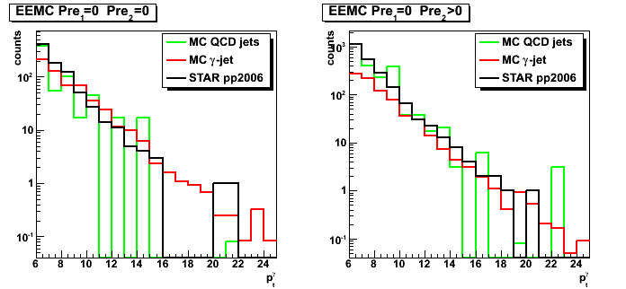
Figure 1: Gamma pt distribution for R_cluster >0.9.
No energy in both pre-shower layer (left plot), and
No energy in pre-shower1 and non-zero energy in pre-shower2 (right plot)
Same figure for R_cluster>0.99 can be found here

Figure 2: Gamma pt distribution for R_cluster >0.9.
No energy in first EEMC pre-shower1 layer (left plot), and
non-zero energy in pre-shower1 (right plot)
For more details (yield, ratios, all pre12 four conditions, etc) see figures 1-3 here.

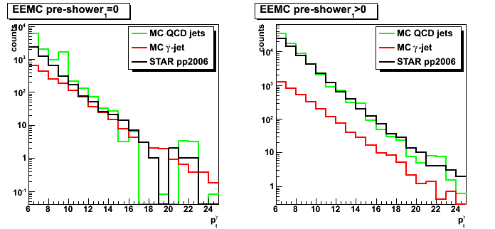
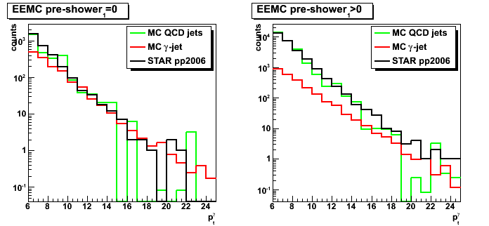
Figure 3: Gamma pt distribution for R_cluster >0.99.
For more details (yield, ratios, all pre12 four conditions, etc) see figures 1-3 here.

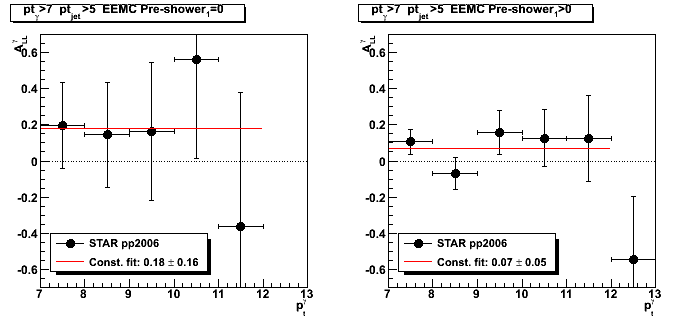
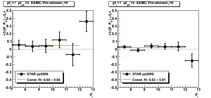
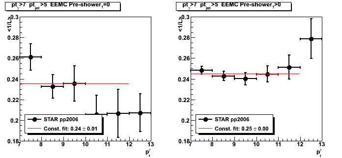
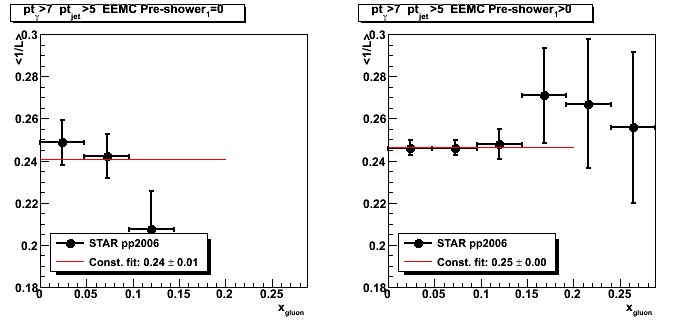
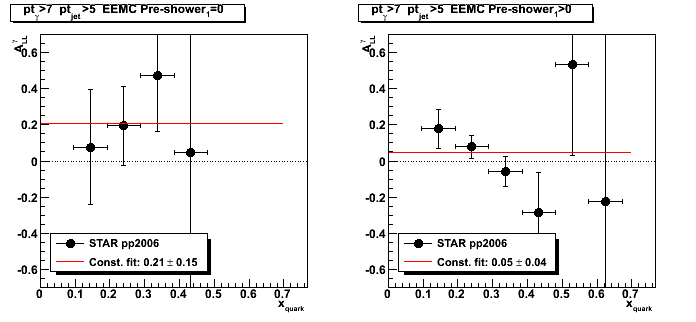
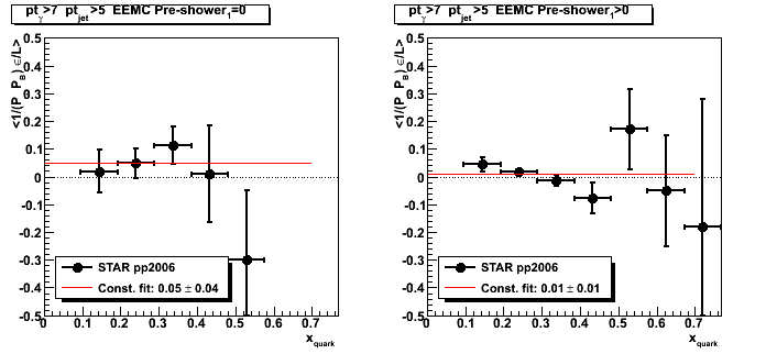
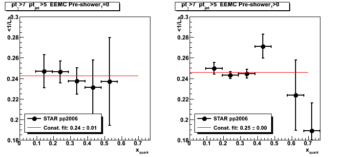
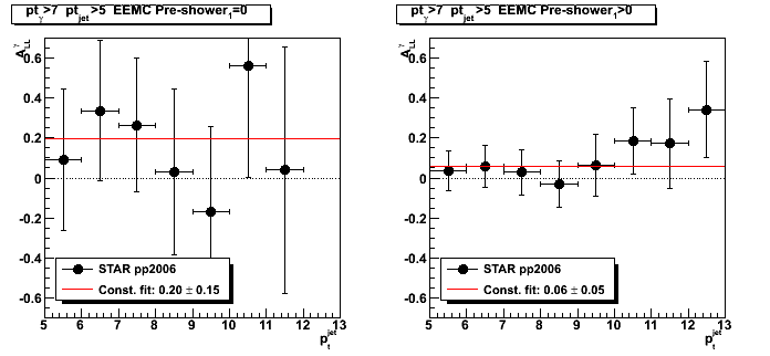
2008.06.10 Gamma-jet candidate longitudinal double spin asymmetry

Ilya Selyuzhenkov June 10, 2008

Note: No background subtraction has been done yet

The case of pre-shower1=0 (left plots) roughly has 1:1 signal to background ratio,
while pre-shower1>0 (right plots) have 1:10 ratio (See MC to data comparison for details).

Data sets:

pp2006 - STAR 2006 pp longitudinal data (~ 3.164 pb^1) after applying gamma-jet isolation cuts,
plus two additional vertex QA cuts:
a) |z_vertex| < 100 and
b) 180 < bbcTimeBin < 300
Polarization fill by fill: blue and yellow
Relative luminosity by polarization fills and runs: relLumi06_070614.txt.gz
Equations used to calculate A_LL from the data: pdf file

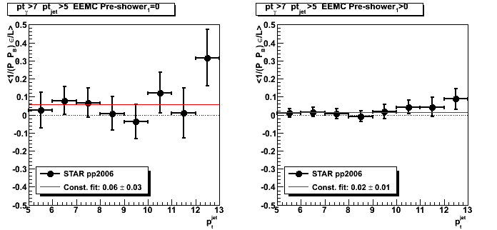
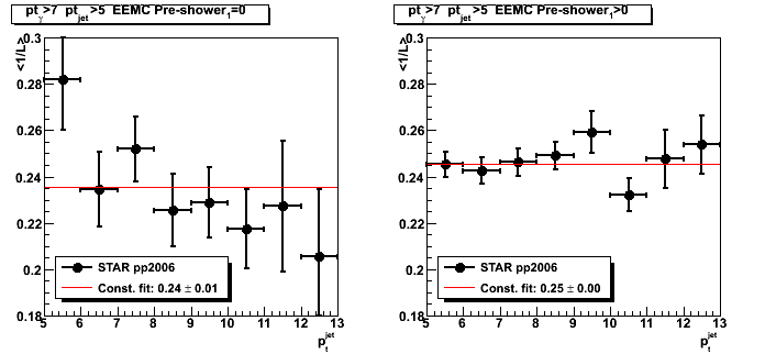
Figure 1: Gamma-jet candidate A_LL vs gamma pt.
Figures for related epsilon_LL and 1/Lum scaled by a factor 10^7
(see pdf/html links above for epsilon_LL and 1/Lum definitions)

Figure 2: Gamma-jet candidate A_LL vs x_gluon.
Figures for related epsilon_LL and 1/Lum scaled by a factor 10^7

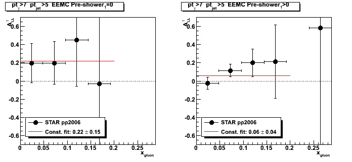
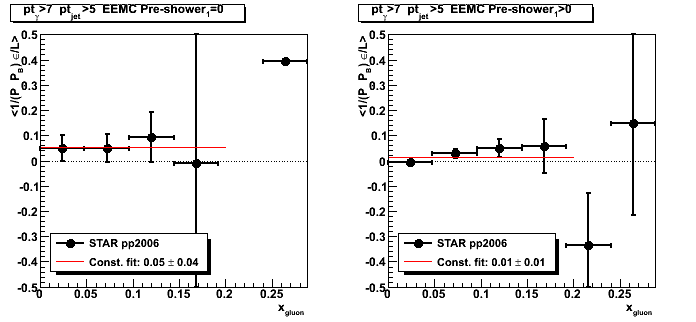
Figure 3: Gamma-jet candidate A_LL vs x_quark.
Figures for related epsilon_LL and 1/Lum scaled by a factor 10^7

Figure 4: Gamma-jet candidate A_LL vs away side jet pt.
Figures for related epsilon_LL and 1/Lum scaled by a factor 10^7

2008.06.18 Photon-jet reconstruction with the EEMC detector (talk at the STAR Collaboration meeting)

Ilya Selyuzhenkov June 18, 2008

Slides

Photon-jet reconstruction with the EEMC detector - Part 1: pdf or odp

Talk outline (preliminary)

Introduction and motivation
Data samples (pp2006, MC gJet, MC QCD bg)
and gamma-jet reconstruction algorithm:
- di-jets, isolation cuts, EEMC 3x3 cluster
- Data sets used and sample EEMC response to a photon candidate
Comparing pp2006 with Monte-Carlo simulations scaled to the same luminosity
(EEMC pre-shower sorting):
EEMC SMD shower shapes from different data samples
(pp2006 and data-driven Monte-Carlo):
- Shower shapes sorted by energy in pre-shower 1 and 2 layers
- pp2006 shower shapes sorted by vertex z, detector eta, phi, pt
Sided residual plots: pp2006 vs data-driven Monte-Carlo
(gammas from eta meson: 3 gaussian fits)
- Sided residual: 2D correlations
- Sided residual: 1D projections
Various cuts study:
- R_cluster cut of 0.99 and 0.9 comparison
  (Cluster energy distribution vs number of EEMC towers fired: Fig.4)
- Charge particle veto and TPC tracking
- Away side jet pt matching
Some QA plots:
- Gamma candidate u- vs. v- plane high strip distribution; x:y position
- Vertex z distribution
A_LL reconstruction technique:
- Method and gamma-jet candidates raw asymmetry
Work in progress... To do list:
- Understading MC background and pp2006 data shower shapes discrepancy
- Implementing sided residual technique with shapes sorted by pre1&2 (eta, sector, etc?)
- Tuning analysis cuts
- Quantifying signal to background ratio
- Background subtraction for A_LL, ...
- What else?
Talk summary

07 Jul

July 2008 posts

2008.07.07 Pre-shower1 < 5MeV cut study

Ilya Selyuzhenkov July 07, 2008

Data sets:

pp2006 - STAR 2006 pp longitudinal data (~ 3.164 pb^1) after applying gamma-jet isolation cuts.
gamma-jet - data-driven Pythia gamma-jet sample (~170K events). Partonic pt range 5-35 GeV.
QCD jets - data-driven Pythia QCD jets sample (~4M events). Partonic pt range 3-65 GeV.

Figure 1: Correlation between 3x3 cluster energy in pre-shower2 vs. pre-shower1 layers

Figure 1a: Distribution of the 3x3 cluster energy in pre-shower1 layer (zoom in for Epre1<0.03 region)
(pp2006 data vs. MC gamma-jet and QCD events)

Figure 2: Shower shapes after pre-shower1 < 5MeV cut.
Shapes are narrower than those without pre1 cut (see Fig. 2)

Figure 3: Gamma pt distribution with pre-shower1 < 5MeV cut.
Compare with distribution withoud pre-shower1 (Fig. 3)

Sided residual (before and after pre-shower1 < 5MeV cut)

Figure 4: Fitted peak vs. maximum sided residual (no pre-shower1 cuts)
Only points for pp2006 data are shown.

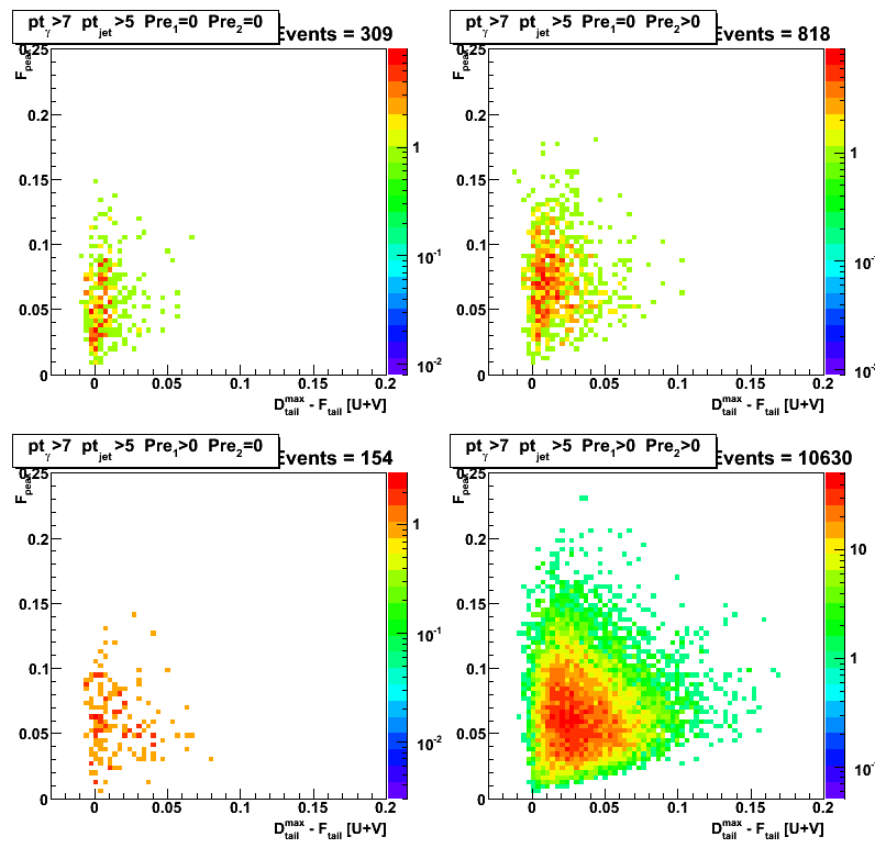
Figure 5: Fitted peak vs. maximum sided residual (after pre-shower1 < 5MeV cut).
Only points for pp2006 data are shown.
Note that distribution for pre1>0,pre2>0 case are narrower
compared to that in Fig.4 (without pre-shower1 cuts).

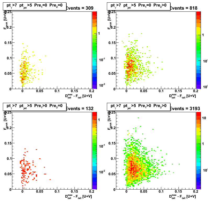
Figure 6: Distribution of maximum sided residual with pre-shower1 < 5MeV cut.

2008.07.16 Gamma-gamma invariant mass cut study

Ilya Selyuzhenkov July 16, 2008

Three data sets:

pp2006 - STAR 2006 pp longitudinal data (~ 3.164 pb^1) after applying gamma-jet isolation cuts.
gamma-jet - data-driven Pythia gamma-jet sample (~170K events). Partonic pt range 5-35 GeV.
QCD jets - data-driven Pythia QCD jets sample (~4M events). Partonic pt range 3-65 GeV.

My simple gamma-gamma finder is trying to
find a second peaks (clusters) in each SMD u and v planes,
match u and v plane high strip intersections,
and calculate the invaraint mass from associated tower energies (3x3 cluster)
according to the energy sharing between SMD clusters.

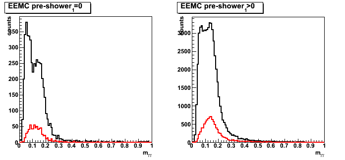
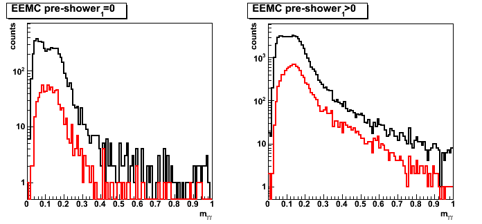
Figure 1: Gamma-gamma invariant mass plot.
Only pp2006 data are shown: black: no pt cuts, red: gamma pt>7GeV and jet pt>5 GeV.
Clear pi0 peak in the [0.1,0.2] invariant mass region.
Same data on the log scale

Gamma pt distributions

Figure 2: Gamma pt distribution (no inv mass cuts).

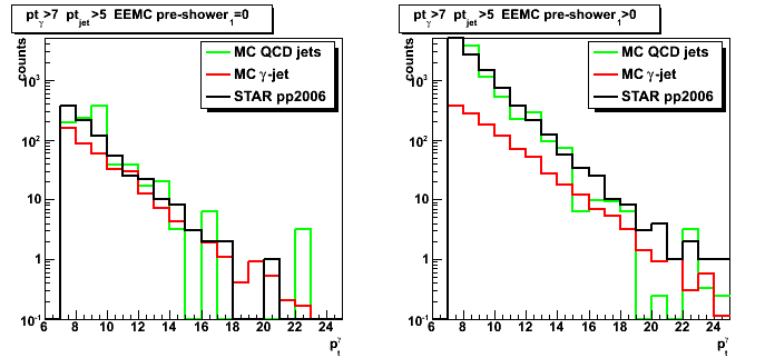
Figure 3: Gamma pt distribution (m_invMass<0.11 or no second peak found).
This cut improves signal to background ratio.

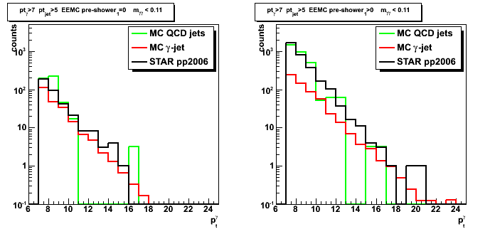
Figure 4: Gamma pt distribution (m_invMass>0.11).
Mostly background events.

Shower shapes

Figure 5: Shower shapes (no pre1 and no invMass cuts).
Good match between shapes in case of no energy in pre-shower1 layer (pre1=0 case).

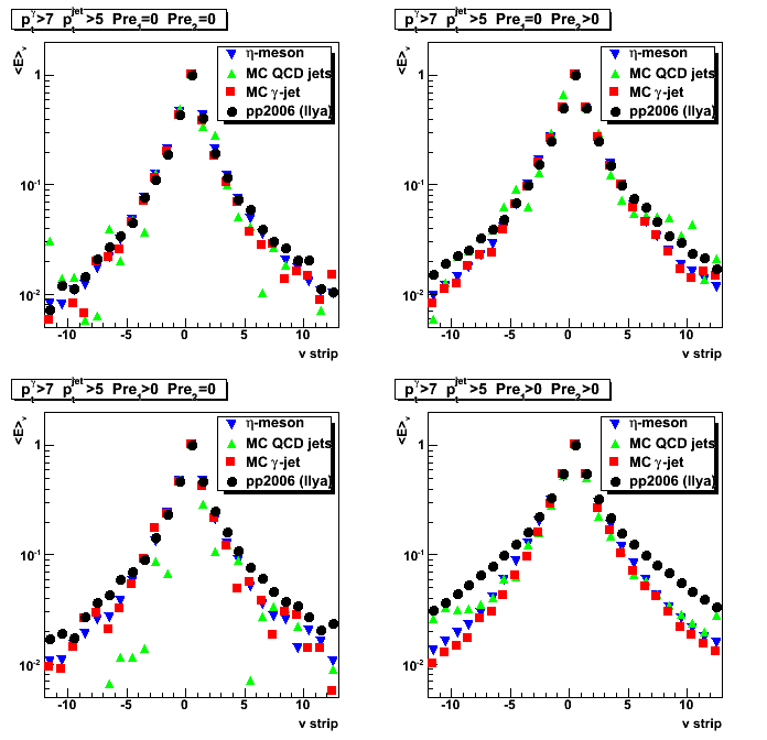
Figure 6: Shower shapes (pre1<5MeV, no invMass cuts).
For pre1&2>0 case shapes getting closer to ech other, but still do not match.

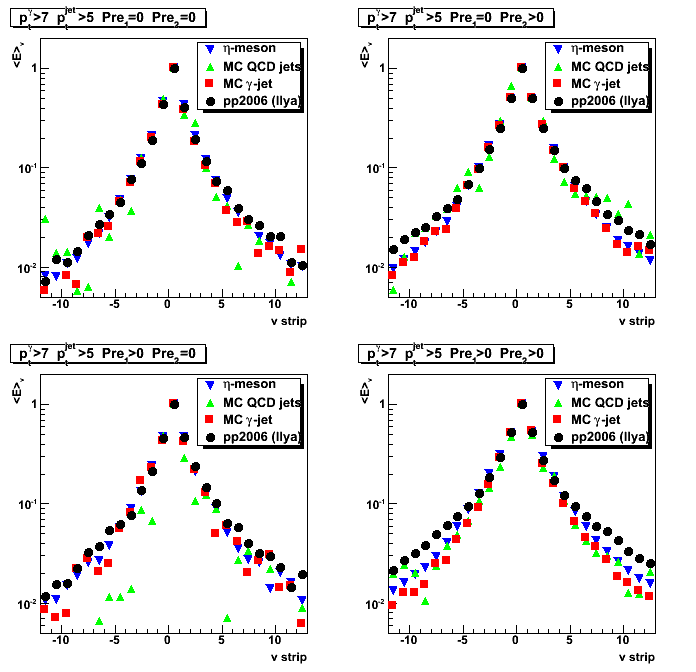
Figure 7: Shower shapes (cuts: pre1<5MeV, invMass<0.11 or no second peak found).
Note, the surprising agreement between eta-meson shapes (blue) and data (black).

Gamma-gamma invariant mass plots

Figure 8: Invariant mass distribution (MC vs. pp2006 data): no pre1 cut

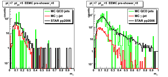
Figure 9: Invariant mass distribution (MC vs. pp2006 data): pre1<5MeV
Left side is the same as in Figure 8

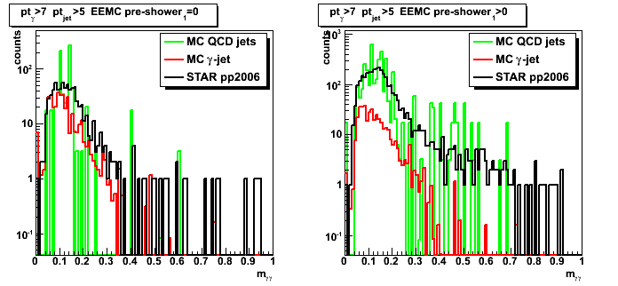
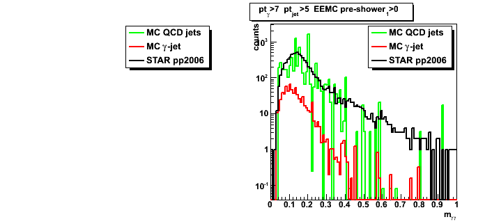
Figure 10: Invariant mass distribution (MC vs. pp2006 data): pre1>5MeV
Left side plot is empty, since there is no events with [pre1=0 and pre1>5MeV]

2008.07.22 Photons from eta-meson: library QA

Ilya Selyuzhenkov July 22, 2008

Shower shapes

Figure 1: Shower shapes: no energy cuts, only 12 strips from peak (left u-plane, right v-plane).

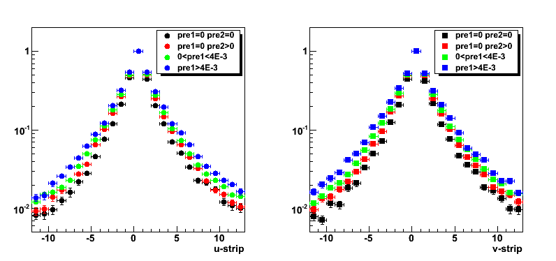
Figure 1a: Shower shapes: no energy cuts, 150 strips from peak (left u-plane, right v-plane).

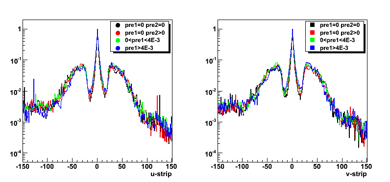
Figure 2: Shower shapes Energy>8GeV (left u-plane, right v-plane).

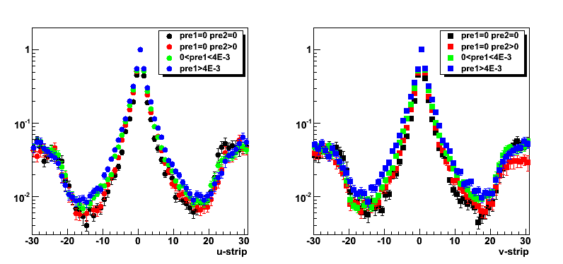
Figure 3: Shower shapes Energy<=8GeV (left u-plane, right v-plane).

One dimensional distributions

Figure 4: Tower energy.

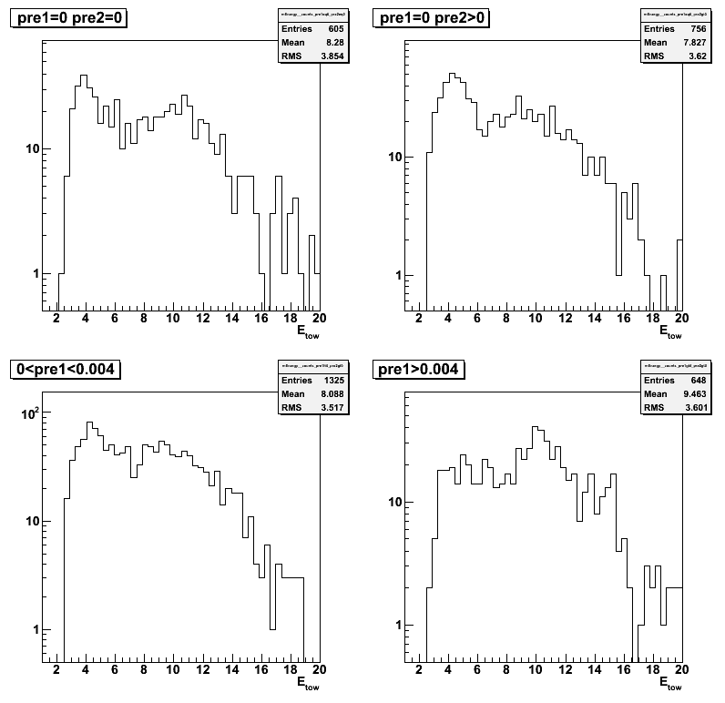
Figure 5: Post-shower energy.

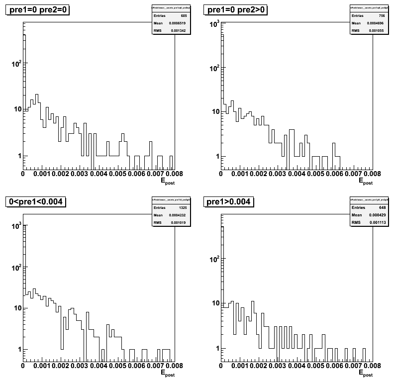
Figure 6: Pre-shower1 energy.

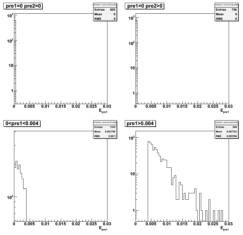
Figure 7: Pre-shower2 energy.

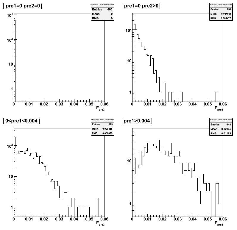
Figure 8: Number of library candidates per sector.

Correlation plots

Figure 9: Transverse momentum vs. energy.

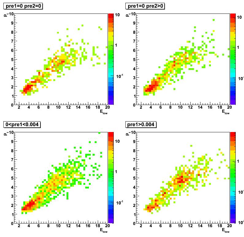
Figure 10: Distance from center of the detector vs. energy.

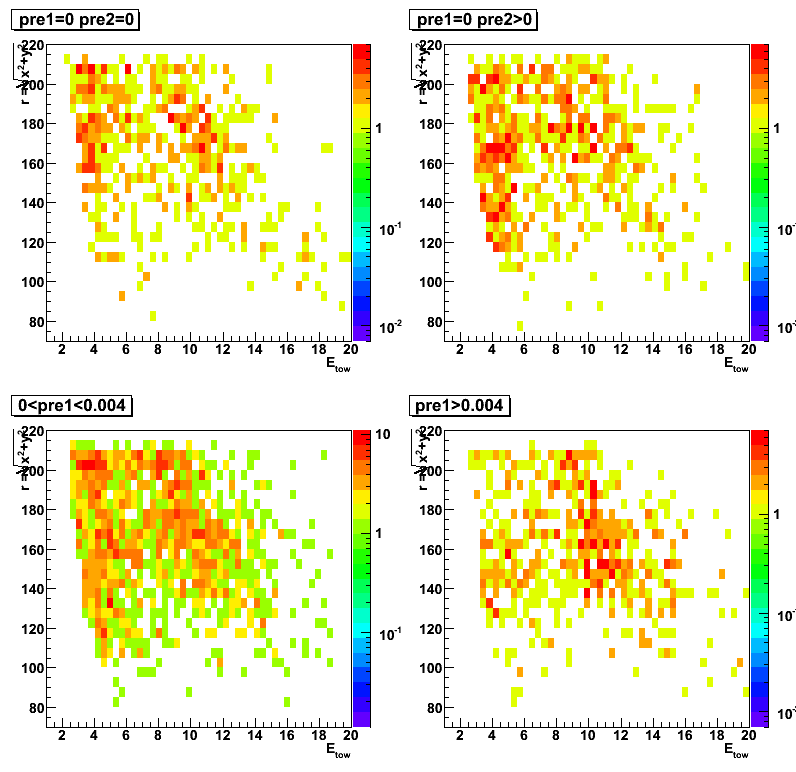
Figure 11: x:y position.

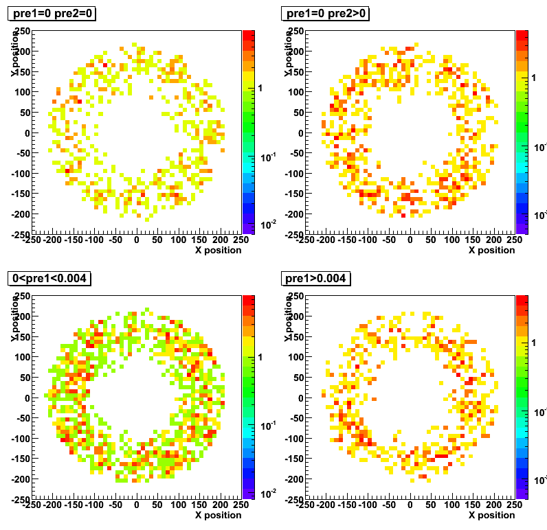
Figure 12: u- vs. v-plane position.

2008.07.29 Shower shape comparison with new dd-library bins

Ilya Selyuzhenkov July 29, 2008

Data sets:

pp2006 - STAR 2006 pp longitudinal data (~ 3.164 pb^1) after applying gamma-jet isolation cuts.
gamma-jet - data-driven Pythia gamma-jet sample (~170K events). Partonic pt range 5-35 GeV.
QCD jets - data-driven Pythia QCD jets sample (~4M events). Partonic pt range 3-65 GeV.

Latest data-driven shower shape replacement library:

Four pre-shower bins: pre1,2=0, pre1=0,pre2>0 pre1<4MeV, pre1>=4MeV
plus two energy bins (E<8GeV, E>=8GeV)

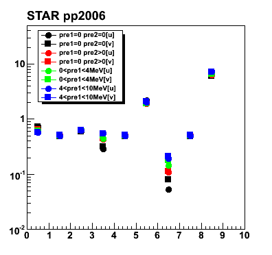
Figure 1: Shower shapes for u-plane [12 strips]
Shower shapes for the library are for the E>8GeV bin.

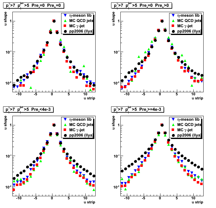
Figure 2: Shower shapes for v-plane [12 strips]

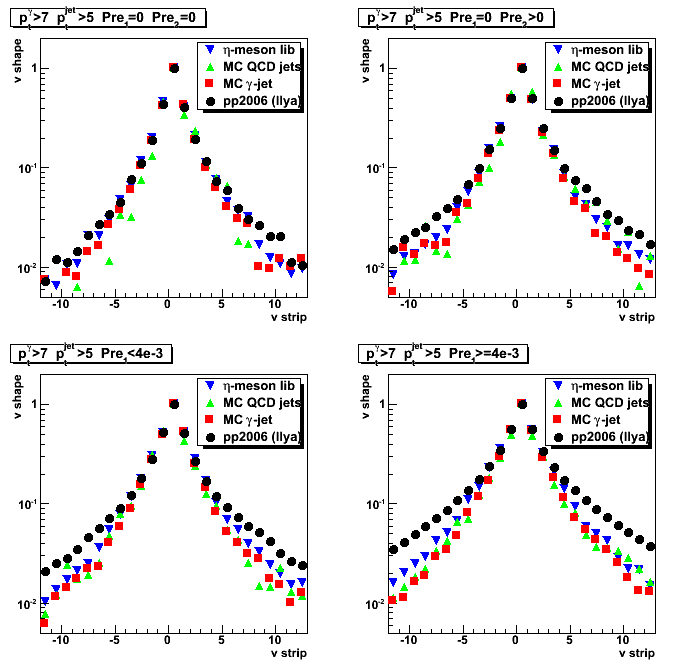
Figure 3: Shower shapes for u-plane [expanded to 40 strips]

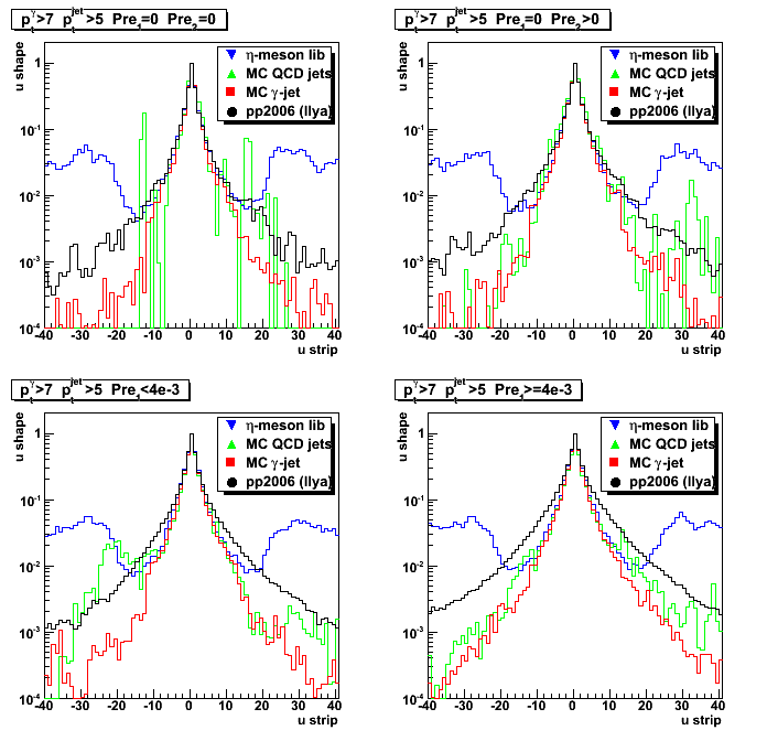
Figure 4: Shower shapes for v-plane [expanded to 40 strips]

08 Aug

August 2008 posts

2008.08.14 Shower shape with bug fixed dd-library

Ilya Selyuzhenkov August 14, 2008

Data sets:

pp2006 - STAR 2006 pp longitudinal data (~ 3.164 pb^1) after applying gamma-jet isolation cuts.
gamma-jet - data-driven Pythia gamma-jet sample (~170K events). Partonic pt range 5-35 GeV.
QCD jets - data-driven Pythia QCD jets sample (~4M events). Partonic pt range 3-65 GeV.

Data-driven maker with bug fixed multi-shape replacement:

Four pre-shower bins: pre1,2=0, pre1=0,pre2>0 pre1<4MeV, pre1>=4MeV
plus two energy bins (E<8GeV, E>=8GeV)

Figure 1: Shower shapes for u-plane [12 strips]
Shower shapes for the library are for the E>8GeV bin.
Open squares and triangles represents raw [without dd-maker]
MC gamma-jet and QCD background shower shapes respectively

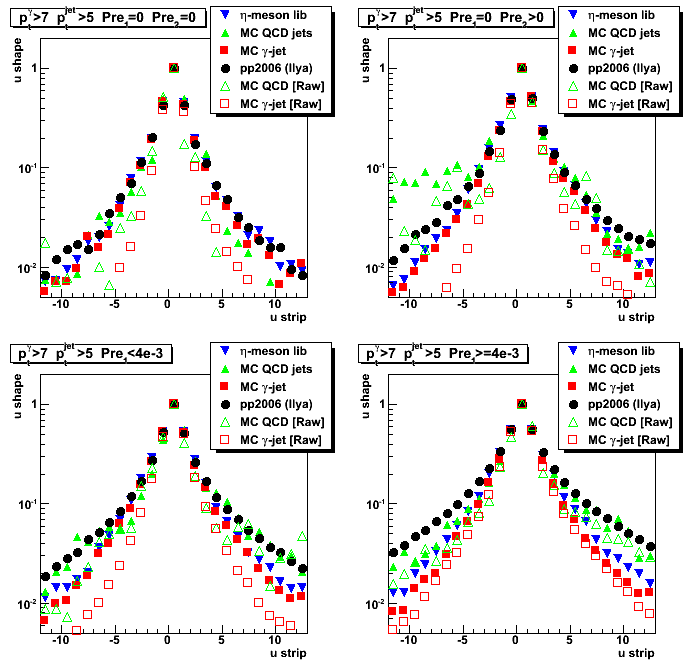
Figure 2: Shower shapes for v-plane [12 strips]

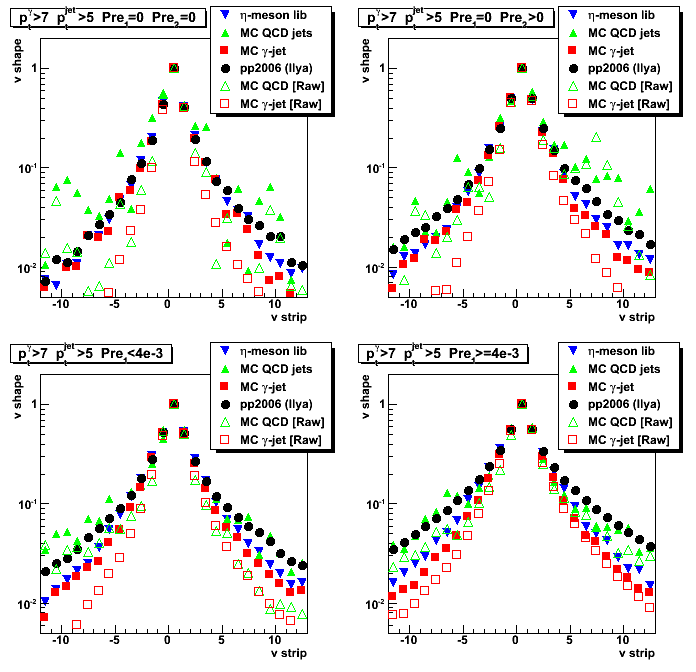
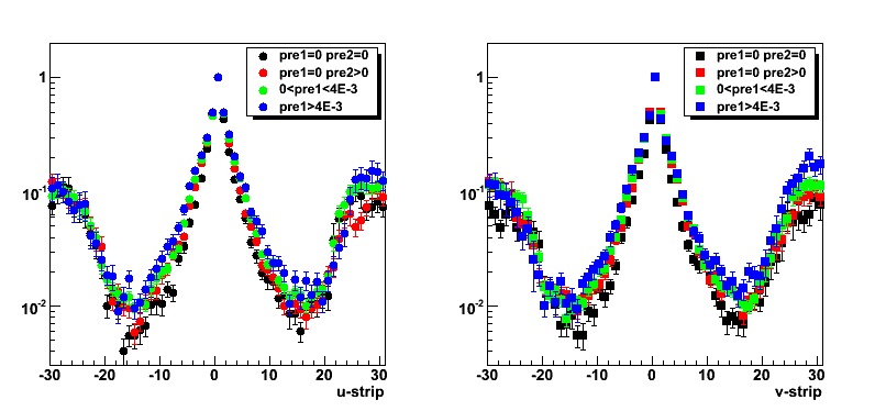
Figure 3: Shower shapes for u-plane [expanded to 40 strips]
Dashed red and green lines represents raw [without dd-maker]
MC gamma-jet and QCD background shower shapes respectively

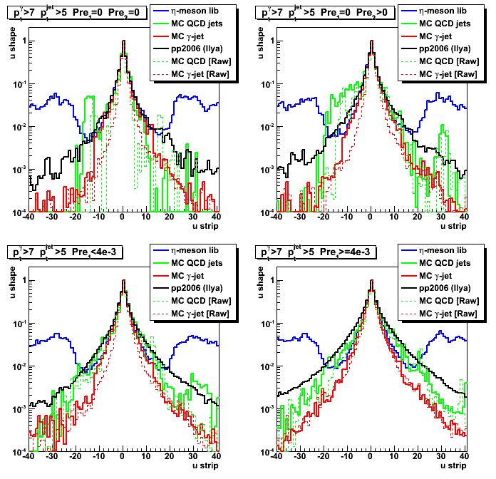
Figure 4: Shower shapes for v-plane [expanded to 40 strips]

2008.08.19 Shower shape from pp2008 vs pp2006 data

Ilya Selyuzhenkov August 19, 2008

Data sets:

pp2006 - STAR 2006 ppProductionLong data (~ 3.164 pb^1)
"eemc-http-mb-l2gamma" trigger after applying gamma-jet isolation cuts.
pp2008 - STAR ppProduction2008 (~ 5.9M events)
"fmsslow" trigger after applying gamma-jet isolation cuts.
[Only ~13 candidates has been selected before pt-cuts]
gamma-jet - data-driven Pythia gamma-jet sample (~170K events). Partonic pt range 5-35 GeV.
QCD jets - data-driven Pythia QCD jets sample (~4M events). Partonic pt range 3-65 GeV.

Note: Due to lack of statistics for 2008 data, no pt cuts applied on gamma-jet candidates for both 2006 and 2008 date.

Figure 1: Shower shapes for u-plane [pp2006 data: eemc-http-mb-l2gamma trigger]

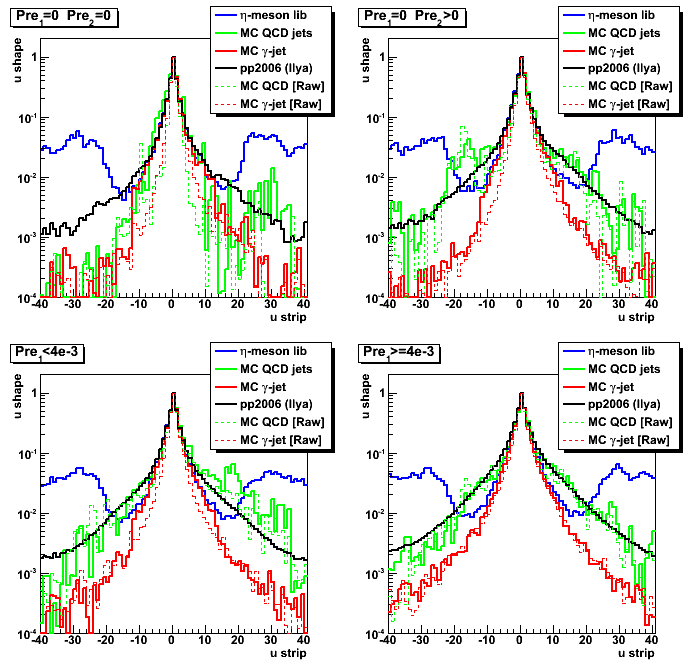
Figure 2: Shower shapes for v-plane [pp2006 data: eemc-http-mb-l2gamma trigger]

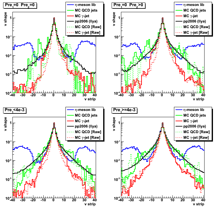
Figure 3: Shower shapes for u-plane [pp2008 data: fmsslow trigger]

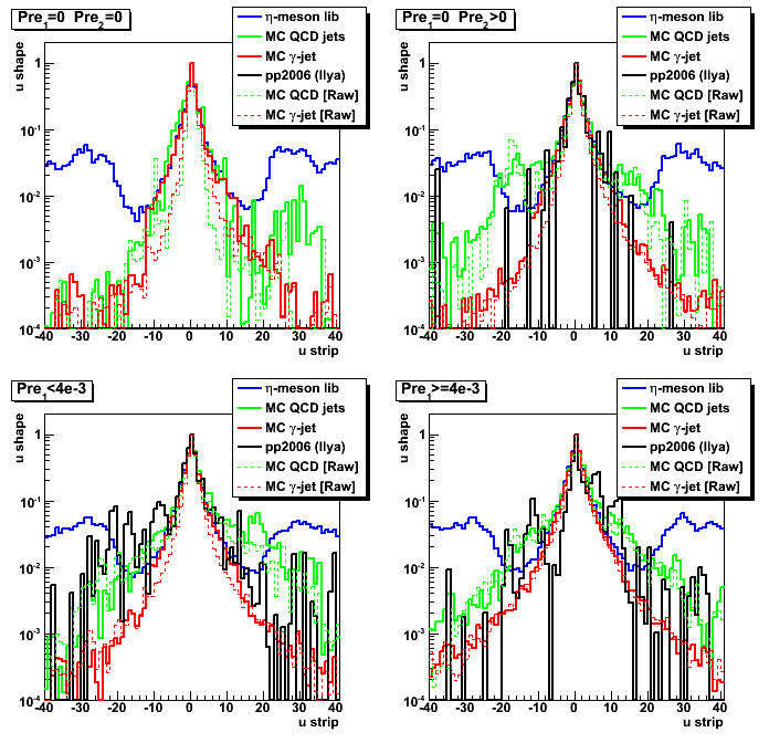
Figure 4: Shower shapes for v-plane [pp2008 data: fmsslow trigger]

2008.08.25 di-jets from pp2008 vs pp2006 data

Ilya Selyuzhenkov August 25, 2008

Data sets:

pp2006 - ppProductionLong [triggerId:137213] (day 136 only)
pp2008 - ppProduction2008 [triggerId:220520] (Jan's set of MuDst from day 047)

Event selection:

Run jet finder and select only di-jet events [adopt jet-finder script from Murad's analysis]
Define jet1 as the jet with largest neutral energy fraction (NEF), and jet2 - the jet with a smaller NEF
Require no EEMC towers associated with jet1
Select trigger (see above) and require vertex to be found

Figure 1: Vertex z distribution (left: pp2008; right: 2006 data)

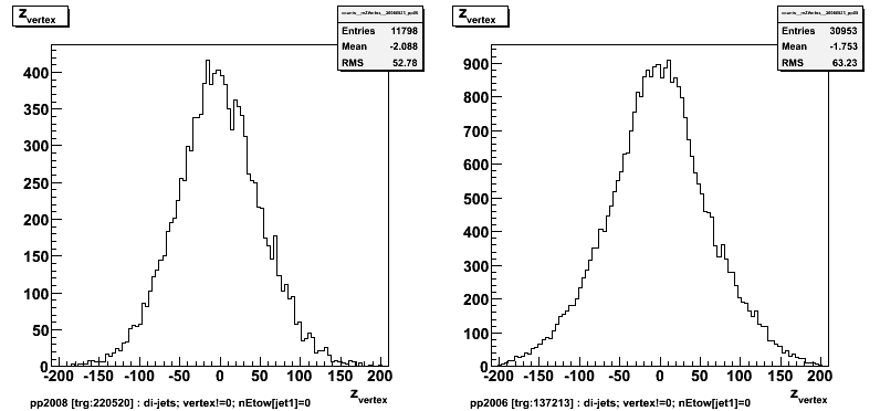
Figure 2: eta vs. phi distribution for the jet1 (jet with largest NEF) .

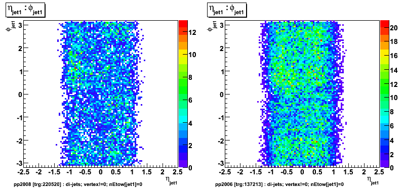
Figure 3: eta vs. z-vertex distribution for the jet1 (jet with largest NEF) .

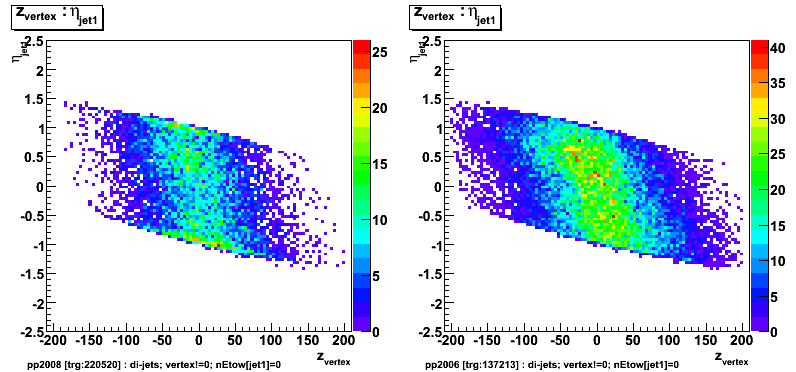
Figure 4: eta vs. z-vertex distribution for the second jet.

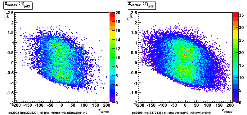
Figure 5: Transverse momentum distribution for jet1.

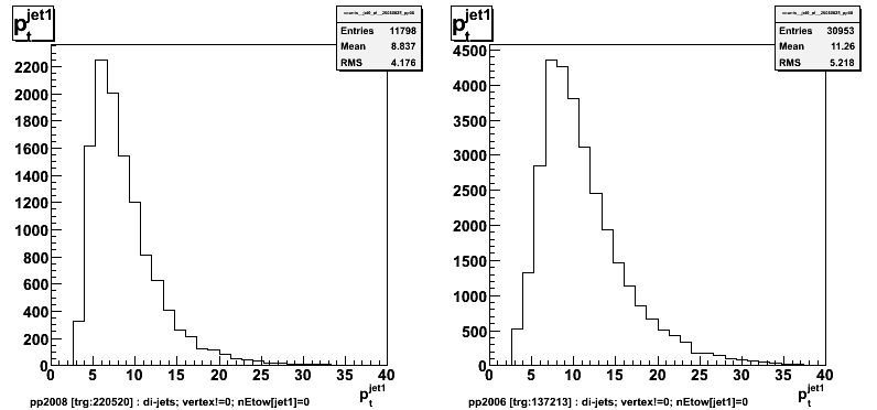
Figure 6: Number of barrel towers associated with jet1.

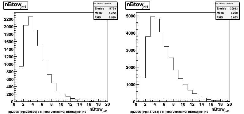
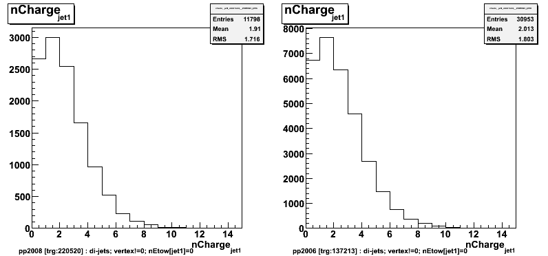
Figure 7: Number of charge tracks associated with jet1.

2008.08.26 Shower shape: more constrains for pre1>4E-3 bin

Ilya Selyuzhenkov August 26, 2008

Data sets:

pp2006 - STAR 2006 pp longitudinal data (~ 3.164 pb^1) after applying gamma-jet isolation cuts.
gamma-jet - data-driven Pythia gamma-jet sample (~170K events). Partonic pt range 5-35 GeV.
QCD jets - data-driven Pythia QCD jets sample (~4M events). Partonic pt range 3-65 GeV.

Data-driven library:

Four pre-shower bins: pre1,2=0, pre1=0,pre2>0 pre1<4MeV, pre1>=4MeV
plus two energy bins (E<8GeV, E>=8GeV)

Figure 1: Pre-shower1 energy distribution for Pre1>4 MeV:
Eta meson library for E>8GeV bin [left] and data vs. MC results [right].

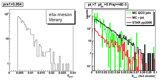
Figure 2: Shower shapes for v-plane [Pre1<10MeV cut]

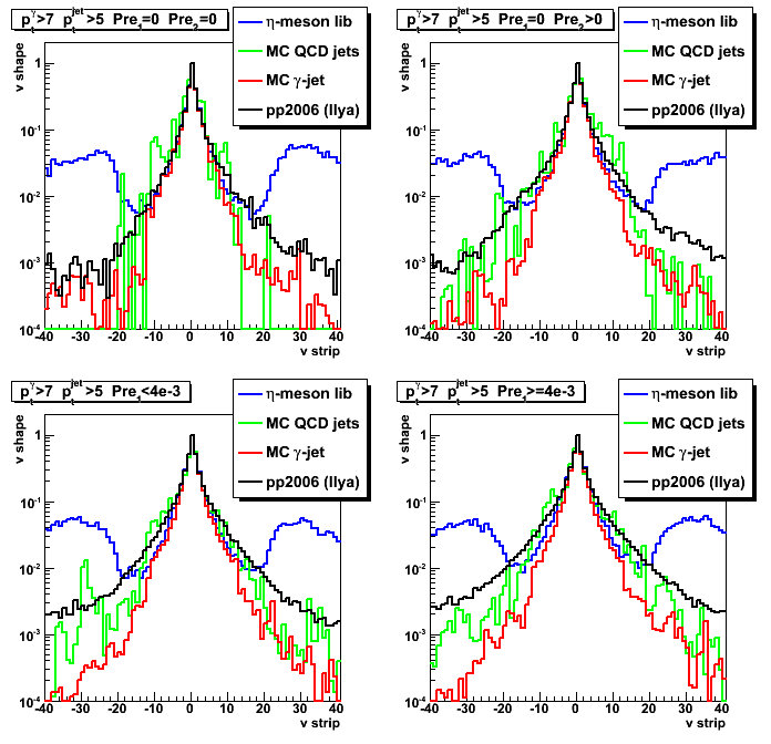
Figure 3: Shower shapes for u-plane [Pre1<10MeV cut]

Maximum side residual plots

Definitions for side residual plot (F_peak, F_tal, D_tail) can be found here
For a moment same 3-gaussian shape is used to fit SMD response for all pre-shower bins.
Algo needs to be updated with a new shapes sorted by pre-shower bins.

Figure 4: Sided residual plot for pp2006 data only [Pre1<10MeV cut]

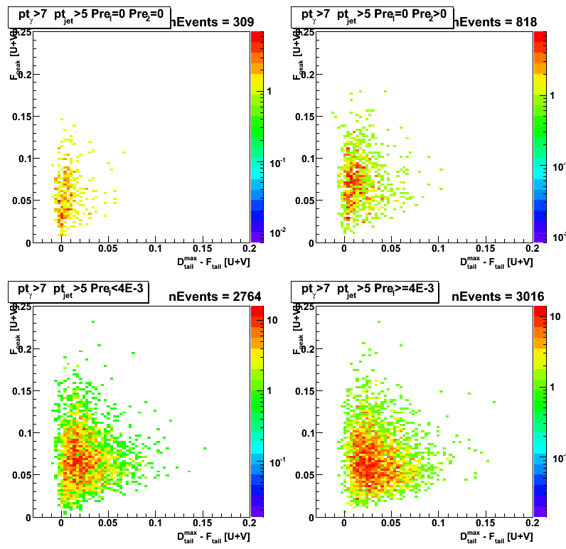
Figure 5: Sided residual projection on "Fitted Peak" axis [Pre1<10MeV cut]

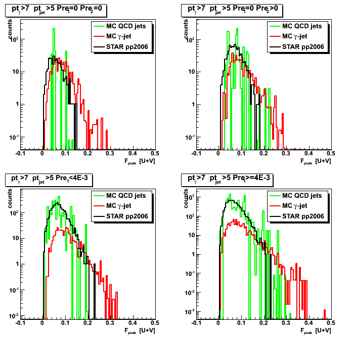
Figure 6: Sided residual projection on "tail difference" axis [Pre1<10MeV cut]

2008.08.27 Gamma-jet candidates detector position for different pre-shower conditions

Ilya Selyuzhenkov August 27, 2008

Data sets:

pp2006 - STAR 2006 pp longitudinal data (~ 3.164 pb^1) after applying gamma-jet isolation cuts.
gamma-jet - data-driven Pythia gamma-jet sample (~170K events). Partonic pt range 5-35 GeV.
QCD jets - data-driven Pythia QCD jets sample (~4M events). Partonic pt range 3-65 GeV.

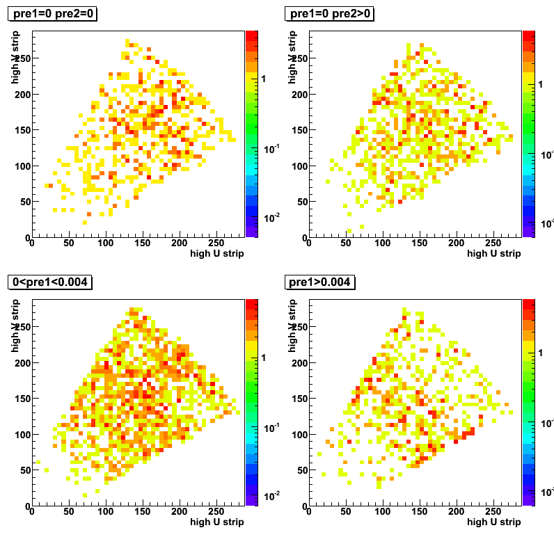
Figure 1: High u vs. v strip id distribution for different pre-shower conditions.
Left column: QCD jets, middle column: gamma-jet, right columnt: pp2006 data

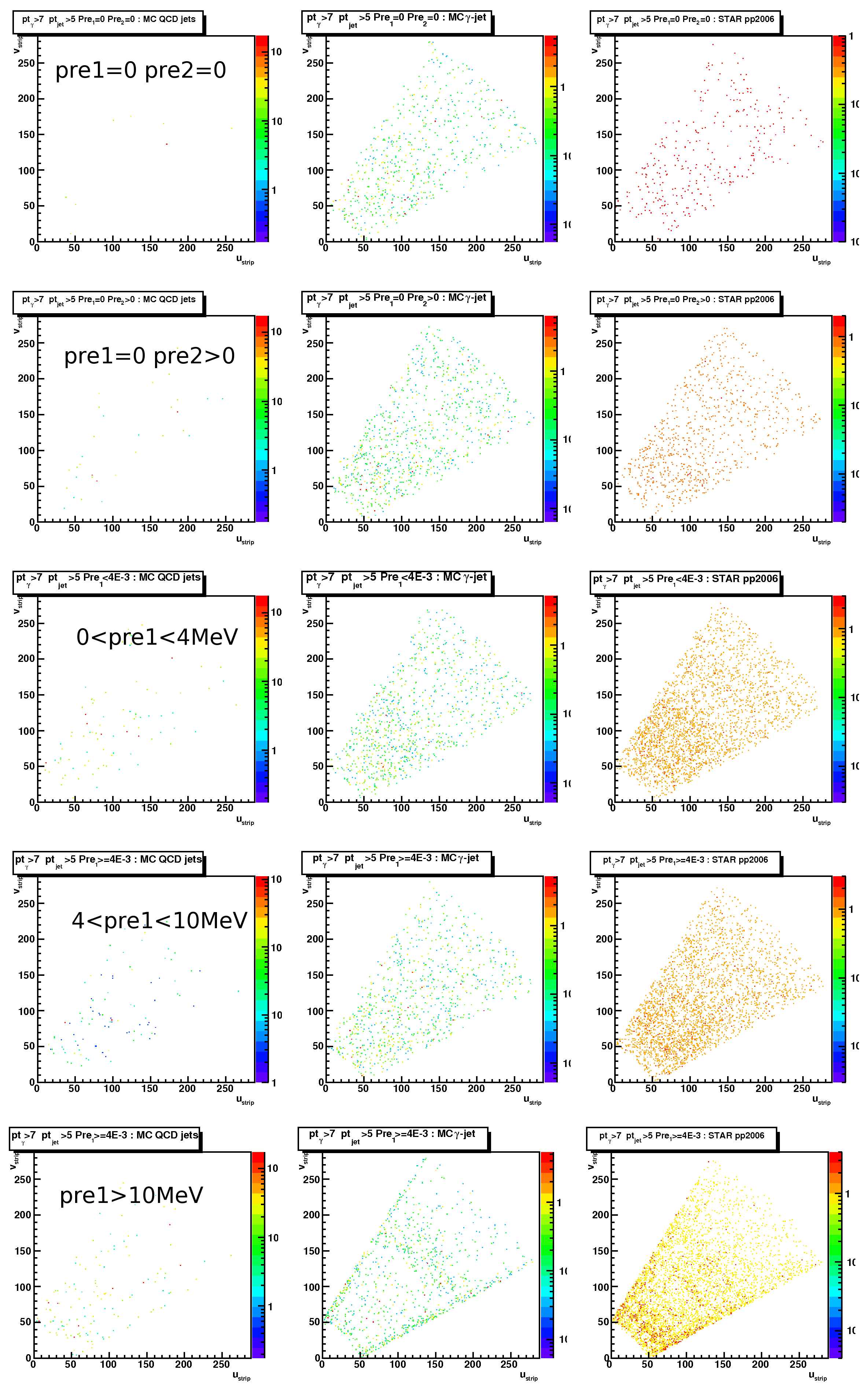
Figure 2: x vs. y position of the gamma-candidate within EEMC detector
for different pre-shower conditions.
Left column: QCD jets, middle column: gamma-jet, right columnt: pp2006 data

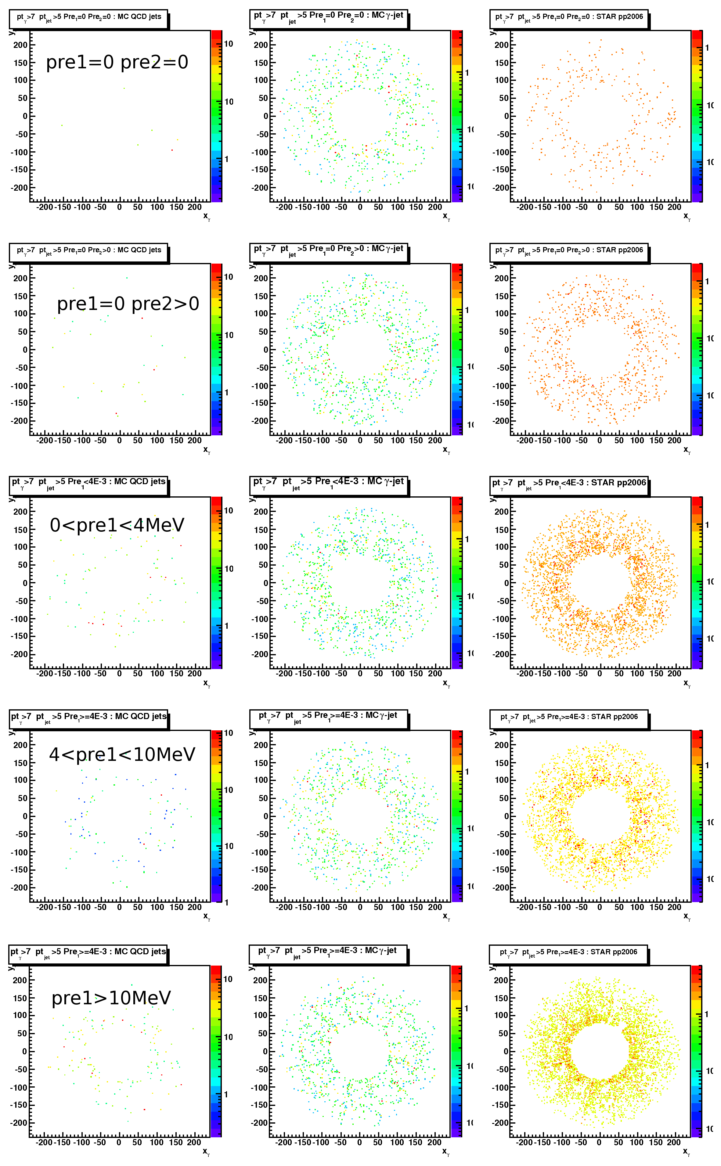
Figure 3:Reconstructed vs. generated (from geant record) gamma pt for the MC gamma-jet sample.
Pre-shower1<10MeV cut applied.

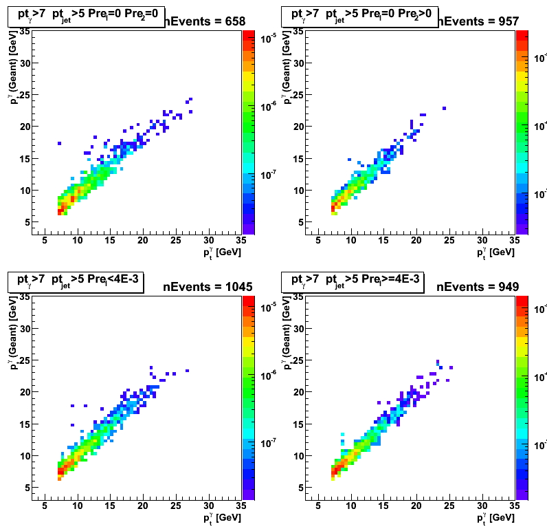
Figure 4:Reconstructed vs. generated (from geant record) gamma eta for the MC gamma-jet sample.
Pre-shower1<10MeV cut applied.

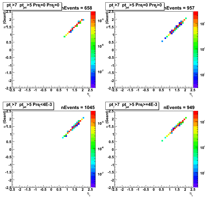
Figure 5:Reconstructed vs. generated (from geant record) gamma phi for the MC gamma-jet sample.
Pre-shower1<10MeV cut applied.

09 Sep

September 2008 posts

2008.09.02 Shower shape fits

Ilya Selyuzhenkov September 02, 2008

Data sets:

pp2006 - STAR 2006 pp longitudinal data (~ 3.164 pb^1) after applying gamma-jet isolation cuts.
gamma-jet - data-driven Pythia gamma-jet sample (~170K events). Partonic pt range 5-35 GeV.
QCD jets - data-driven Pythia QCD jets sample (~4M events). Partonic pt range 3-65 GeV.

Shower shape fitting procedure:

Fit with single Gaussian shape using 3 highest strips
Fit with double Gaussian using 5 strips from each side of the peak [11 strips total]
First Gaussian parameters are fixed from the step above
Re-fit with double Gaussian with initial parameters from step 2 above
Fit with triple Gaussian [fit range varies from 9 to 15 strips, default is 12 strips, see below]
Initial parameters for the first two Gaussian are fixed from step 3 above
Fit with triple Gaussian with initial parameters from step 4 above
(releasing all parameters except mean values)

Fitting function "[0]*(exp ( -0.5*((x-[1])/[2])**2 )+[3]*exp ( -0.5*((x-[4])/[5])**2 )+[6]*exp ( -0.5*((x-[7])/[8])**2 ))"

Fit results for MC gamma-jet data sample

Figure 1: MC gamma-jet shower shapes and fits for u-plane
Results from single, double and triple Gaussian fits (using from 9 to 15 strips) are shown.

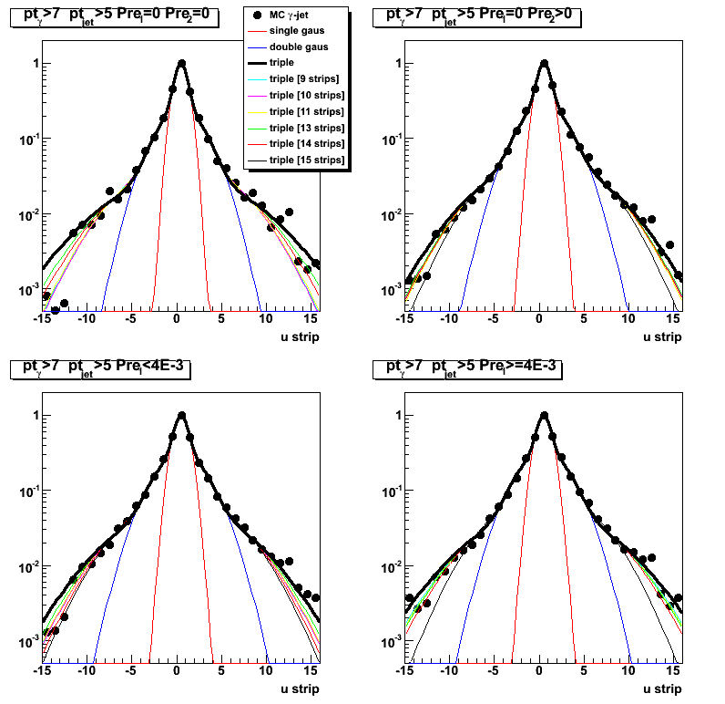
Figure 2: Same as figure 1. but from v-plane

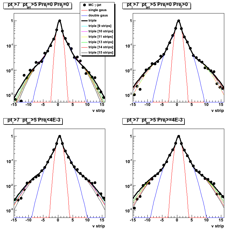
Figure 3: MC gamma-jet results using triple Gaussian fits within 12 strips from a peak.
Left: u-plane. Right: v-plane

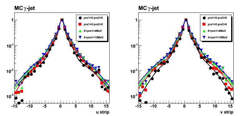
Figure 4: Combined fit results from MC gamma-jet sample

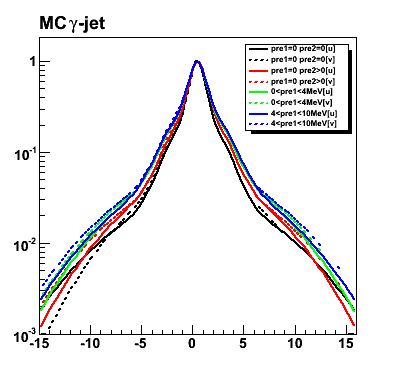
Figure 5: Fitting parameters [see equation for the fit function above].
Note, that parameters 1, 4, and 7 (peak position) has the same value.

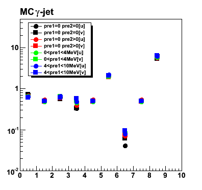
Numerical fit results:

pre1=0 pre2=0 [u]: 0.602039*((exp(-0.5*sq((x-0.491324)/0.605927))+(0.578161*exp(-0.5*sq((x-0.491324)/2.05454))))+(0.0937517*exp(-0.5*sq((x-0.491324)/6.37656))))
pre1=0 pre2=0 [v]: 0.729744*((exp(-0.5*sq((x-0.480945)/0.621631))+(0.327792*exp(-0.5*sq((x-0.480945)/2.01717))))+(0.0410935*exp(-0.5*sq((x-0.480945)/6.49599))))
pre1=0 pre2>0 [u]: 0.725212*((exp(-0.5*sq((x-0.474451)/0.560416))+(0.3332*exp(-0.5*sq((x-0.474451)/1.91957))))+(0.0611053*exp(-0.5*sq((x-0.474451)/5.34357))))
pre1=0 pre2>0 [v]: 0.686446*((exp(-0.5*sq((x-0.536662)/0.650485))+(0.388429*exp(-0.5*sq((x-0.536662)/1.99118))))+(0.0712328*exp(-0.5*sq((x-0.536662)/5.64637))))
0 <4MeV [u]: 0.612486*((exp(-0.5*sq((x-0.485717)/0.592415))+(0.55846*exp(-0.5*sq((x-0.485717)/1.87214))))+(0.0749598*exp(-0.5*sq((x-0.485717)/6.12462))))
0 <4MeV [v]: 0.651584*((exp(-0.5*sq((x-0.486876)/0.652023))+(0.450767*exp(-0.5*sq((x-0.486876)/2.07667))))+(0.0864232*exp(-0.5*sq((x-0.486876)/5.84357))))
4 <10MeV [u]: 0.621905*((exp(-0.5*sq((x-0.496841)/0.632917))+(0.512575*exp(-0.5*sq((x-0.496841)/1.97482))))+(0.0927374*exp(-0.5*sq((x-0.496841)/6.10844))))
4 <10MeV [v]: 0.634943*((exp(-0.5*sq((x-0.505378)/0.660763))+(0.480929*exp(-0.5*sq((x-0.505378)/2.17312))))+(0.0788037*exp(-0.5*sq((x-0.505378)/6.21667))))

Fit results for pp2006 gamma-jet candidates

Figure 6: Same as Fig. 3, but for gamma-jet candidates from pp2006 data

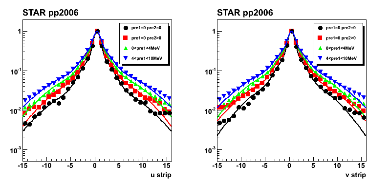
Figure 7: Same as Fig. 5, but for gamma-jet candidates from pp2006 data

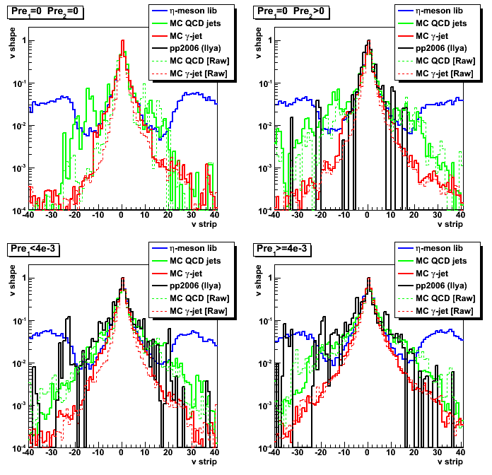
2008.09.09 Maximum sided residual with shower shapes sorted by uv- and pre-shower bins

Ilya Selyuzhenkov September 09, 2008

Data sets:

pp2006 - STAR 2006 pp longitudinal data (~ 3.164 pb^1) after applying gamma-jet isolation cuts.
gamma-jet - data-driven Pythia gamma-jet sample (~170K events). Partonic pt range 5-35 GeV.
QCD jets - data-driven Pythia QCD jets sample (~4M events). Partonic pt range 3-65 GeV.

Procedure to calculate maximum sided residual:

For each event fit SMD u and v energy distributions with
triple Gaussian functions from shower shapes analysis:

[0]*(exp(-0.5*((x-[1])/[2])**2)+[3]*exp(-0.5*((x-[1])/[4])**2)+[6]*exp(-0.5*((x-[1])/[5])**2))
Fit parameters sorted by various pre-shower conditions and u and v-planes can be found here
There are only two free parameters in a final fit: overall amplitude [0] and mean value [1]
Fit range is +-2 strips from the high strip (5 strips total).
Integrate energy from a fit within +-2 strips from high strip.
This is our peak energy from fit, F_peak.
Calculate tail energies on left and right sides from the peak for both data, D_tail, and fit, F_tail.
Tails are integrated up to 30 strips excluding 5 highest strips.
Determine maximum difference between D_tail and F_tail:
max(D_tail-F_tail). This is our maximum sided residual.
Plot F_peak vs. max(D_tail-F_tail). This is sided residual plot.
(implementation for this item is in progress)
Based on MC gamma-jet sided residual plot find a line (some polynomial function)
which will serve as a cut to separate signal and background.
Use that cut line to calculate signal to background ratio
and apply it for the real data analysis.

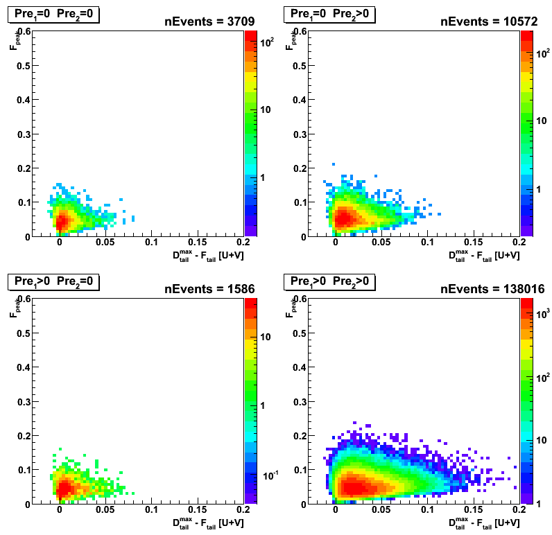
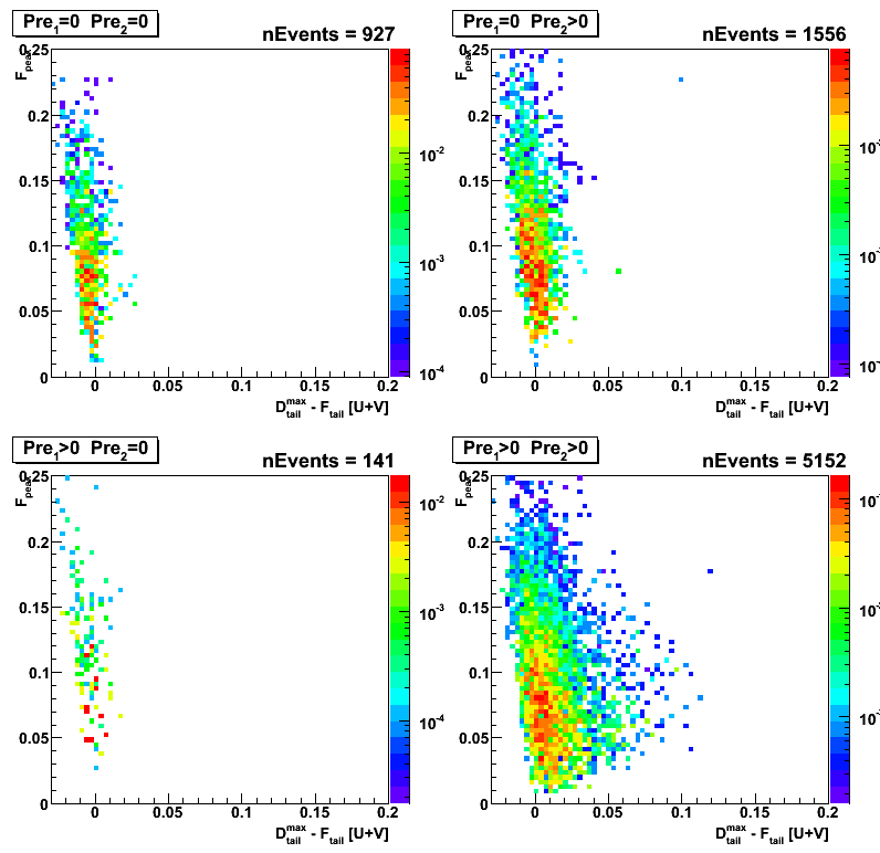
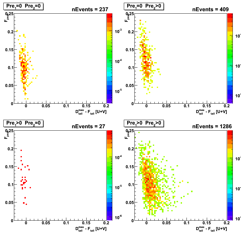
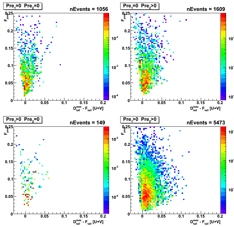
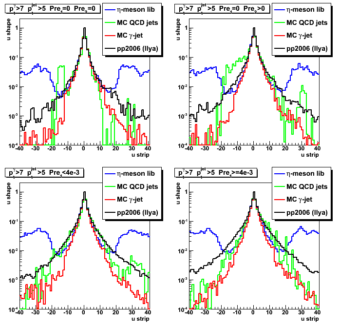
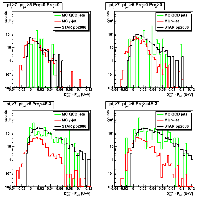
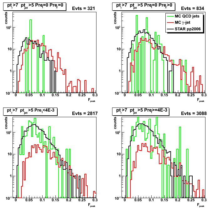
Figure 1: Maximum sided residual plots for different data sets and various pre-shower condition.
Columns [data sets]: 1. MC QCD background; 2. gamma-jet; 3. pp2006 data
Rows [pre-shower bins]: 1. pre1=0 pre2=0; 2. pre1=0, pre2>0; 3. 0<pre1<4MeV; 4. 4<pre1<10MeV
Results from u and v plane are combined as [U+V]/2

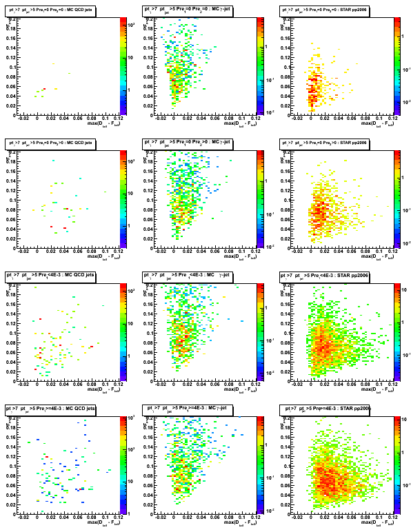
Figure 2: max(D_tail-F_tail) distribution (projection on horizontal axis from Fig.1)
Some observations:
Results for pp2006 and MC gamma-jet are consistent for pre1=0 pre2=0 case (upper left plot)
Results for pp2006 and MC QCD background jets are also in agrees for pre1>0 case (lower left and right plots)

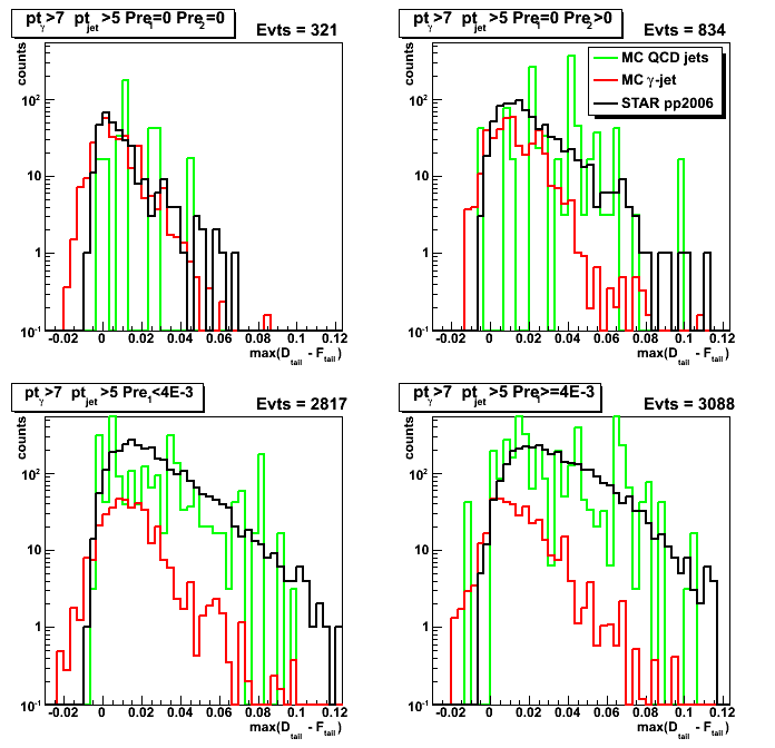
Figure 3: F_peak distribution (projection on vertical axis from Fig.1)

2008.09.16 QA plots for maximum sided residual (obsolete)

Ilya Selyuzhenkov September 16, 2008

These results are obsolete.
Please use this link instead

Data sets:

pp2006 - STAR 2006 pp longitudinal data (~ 3.164 pb^1) after applying gamma-jet isolation cuts.
gamma-jet - data-driven Pythia gamma-jet sample (~170K events). Partonic pt range 5-35 GeV.
QCD jets - data-driven Pythia QCD jets sample (~4M events). Partonic pt range 3-65 GeV.

Notations used in the plots:

Fit peak energy:
F_peak - integral within +-2 strips from maximum strip
Maximum strip determined by fitting procedure.
Float value converted ("cutted") to integer value.
Data peak energy:
D_peak - energy sum within +-2 strips from maximum strip (the same strip Id as for F_peak).
Data tails:
D_tail^left and D_tail^right.
Energy sum from 3rd strip up to 30 strips on the
left and right sides from maximum strip (excludes strips which contributes to D_peak)
Fit tails:
F_tail^left and F_tail^right.
Same definition as for D_tail, but integrals are calculated from a fit function.
Maximum sided residual:
max(D_tail-F_tail)
Maximum of the data minus fit energy on the left and right sides from the peak.

Figure 1: D_peak from [U+V]/2.

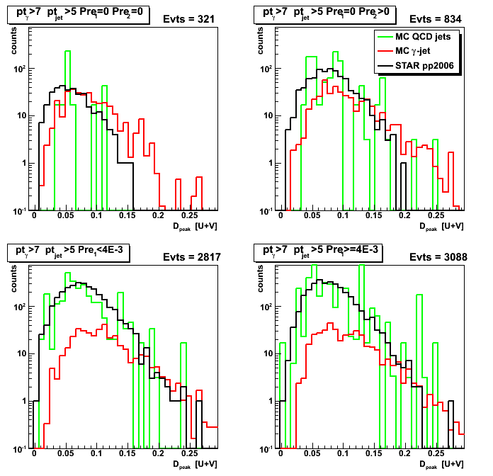
Figure 2: U/V asymmetry for D_peak: [U-V]/[U+V]

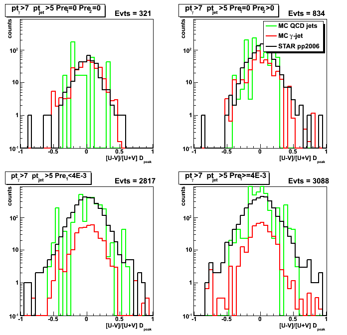
Figure 3: F_peak from [U+V]/2.

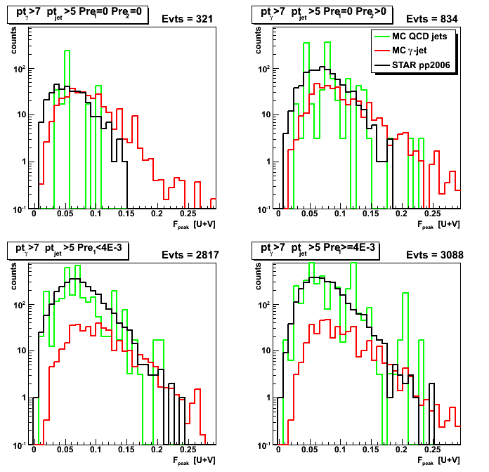
Figure 4: U/V asymmetry for F_peak: [U-V]/[U+V]

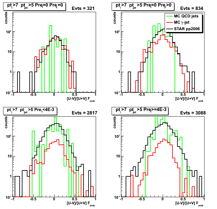
Figure 5: (D_peak - F_peak)/D_peak asymmetry

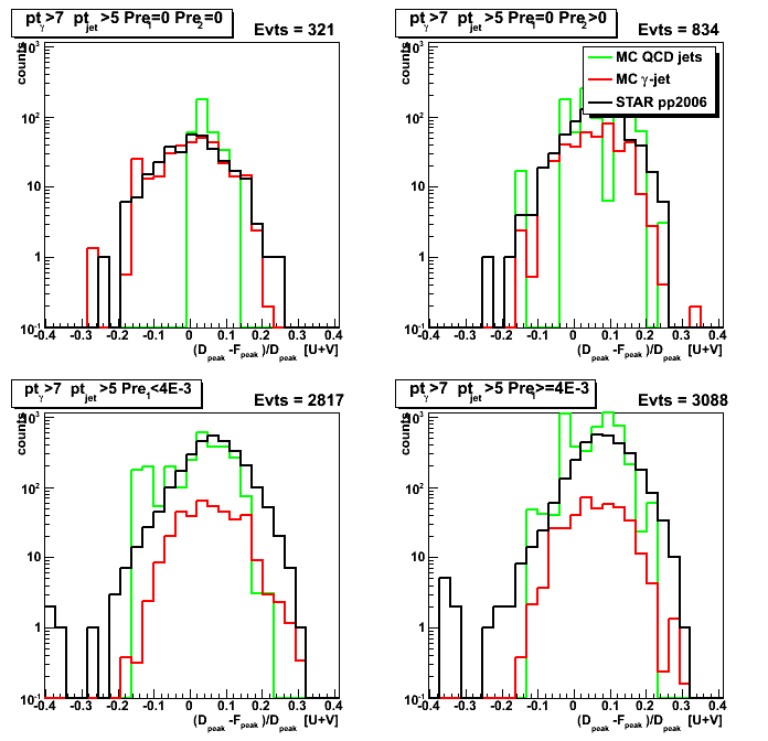
Figure 6: Maximum sided residual from V vs. U plane.

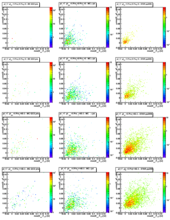
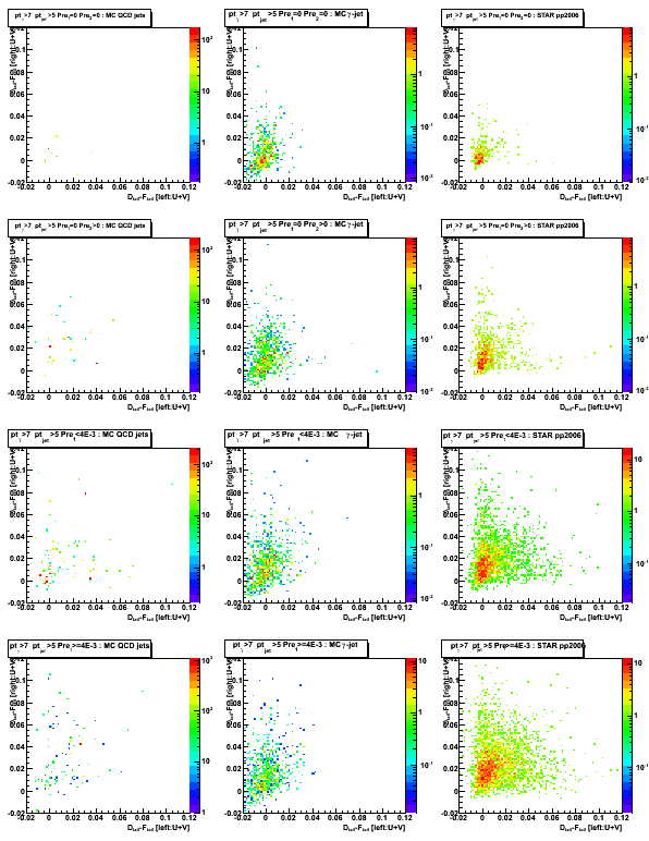
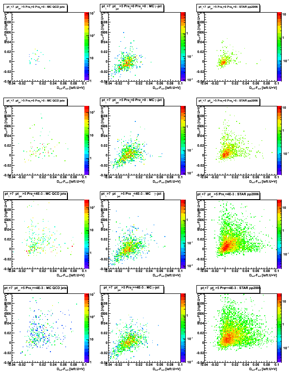
Figure 7: (D_tail-F_tail)^right vs. (D_tail-F_tail)^left

2008.09.23 QA plots for maximum sided residual (bug fixed update)

Ilya Selyuzhenkov September 23, 2008

Data sets:

pp2006 - STAR 2006 pp longitudinal data (~ 3.164 pb^1)
after applying gamma-jet isolation cuts (note: R_cluster > 0.9 is used below).
gamma-jet - data-driven Pythia gamma-jet sample (~170K events). Partonic pt range 5-35 GeV.
QCD jets - data-driven Pythia QCD jets sample (~4M events). Partonic pt range 3-65 GeV.

Notations used in the plots:

Fit peak energy:
F_peak - integral within +-2 strips from maximum strip
Maximum strip determined by fitting procedure.
Float value converted ("cutted") to integer value.
Data peak energy:
D_peak - energy sum within +-2 strips from maximum strip (the same strip Id as for F_peak).
Data tails:
D_tail^left and D_tail^right.
Energy sum from 3rd strip up to 30 strips on the
left and right sides from maximum strip (excludes strips which contributes to D_peak)
Fit tails:
F_tail^left and F_tail^right.
Same definition as for D_tail, but integrals are calculated from a fit function.
Maximum sided residual:
max(D_tail-F_tail)
Maximum of the data minus fit energy on the left and right sides from the peak.

Figure 1: D_peak from [U+V]/2.

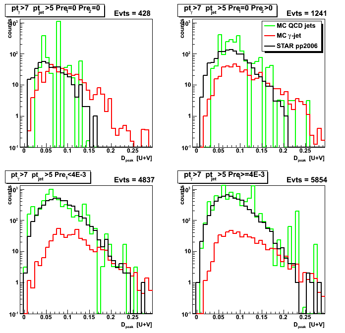
Figure 2: (D_peak - F_peak)/D_peak asymmetry

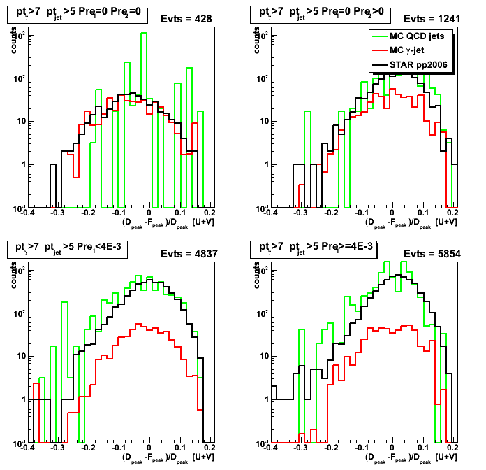
Figure 3: Maximum sided residual from V vs. U plane.

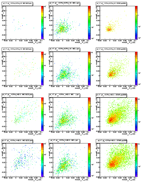
Figure 4: (D_tail-F_tail)^right. (D_tail-F_tail)^left

2008.09.23 Right-left SMD tail asymmetries

Ilya Selyuzhenkov September 23, 2008

Figure 1: D_peak vs. [right-left] D_tail

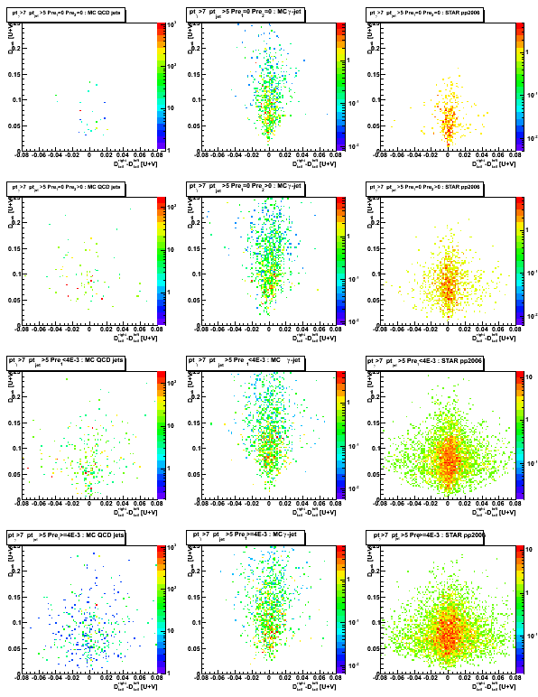
Figure 2: [right-left]/[right-+left] D_tail

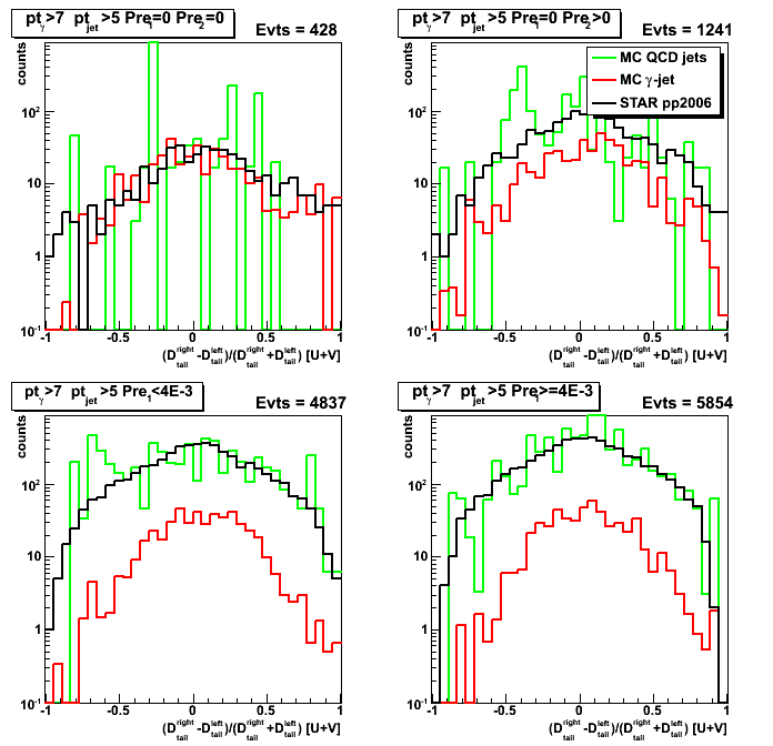
2008.09.23 Sided residual plot projection: toward s/b efficency/rejection plot

Ilya Selyuzhenkov September 23, 2008

Data sets:

pp2006 - STAR 2006 pp longitudinal data (~ 3.164 pb^1)
after applying gamma-jet isolation cuts (note: R_cluster > 0.9 is used below).
gamma-jet - data-driven Pythia gamma-jet sample (~170K events). Partonic pt range 5-35 GeV.
QCD jets - data-driven Pythia QCD jets sample (~4M events). Partonic pt range 3-65 GeV.

Notations used in the plots:

Fit peak energy:
F_peak - integral within +-2 strips from maximum strip
Maximum strip determined by fitting procedure.
Float value converted ("cutted") to integer value.
Data peak energy:
D_peak - energy sum within +-2 strips from maximum strip (the same strip Id as for F_peak).
Data tails:
D_tail^left and D_tail^right.
Energy sum from 3rd strip up to 30 strips on the
left and right sides from maximum strip (excludes strips which contributes to D_peak)
Fit tails:
F_tail^left and F_tail^right.
Same definition as for D_tail, but integrals are calculated from a fit function.
Maximum sided residual:
max(D_tail-F_tail)
Maximum of the data minus fit energy on the left and right sides from the peak.

Maximum sided residual: MC vs. data comparison

Figure 1: Maximum sided residual plot
Top get more statistics for MC QCD sample plot is redone with a softer R_cluster > 0.9 cut

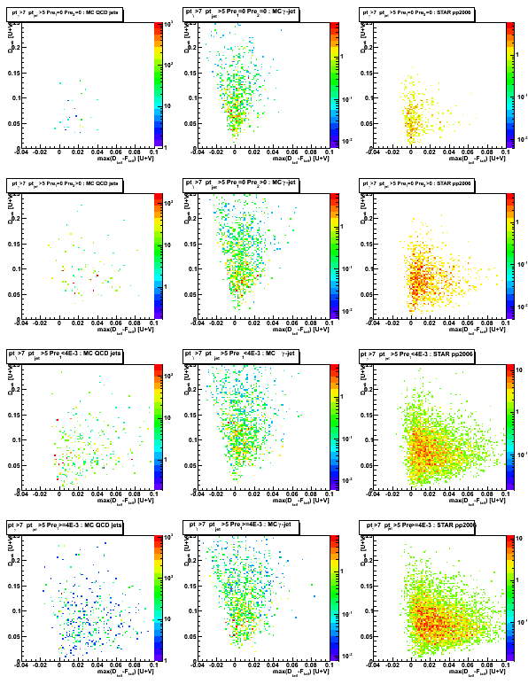
Figure 2: D_peak (projection on vertical axis for Fig. 1)
Upper left plot (no pre-shower fired case) reveals some difference
between MC gamma-jet and pp2006 data at lower D_peak values.
This difference could be due to background contribution at low energies.
Still needs more statistics for MC QCD jet sample to confirm that statement.

Figure 3: max(D_tail-F_tail) (projection on horisontal axis for Fig. 1)
One can get an idea of signal/background separation (red vs. black) depending on pre-shower condition.

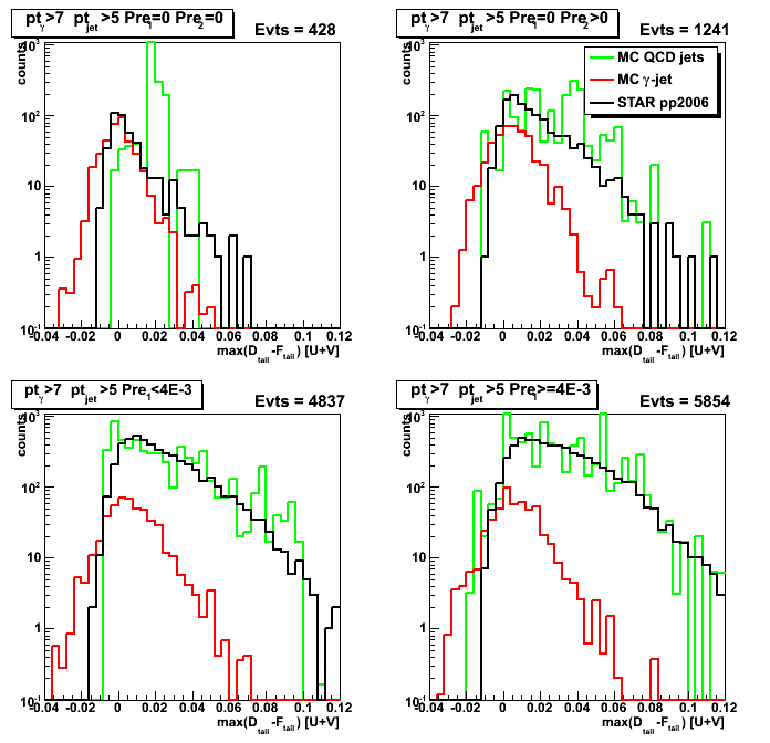
Figure 4: Mean < max(D_tail-F_tail) > vs. D_peak (profile on vertical axis from Fig. 1)
For gamma-jet sample average sided residual is independent on D_peak energy
and has a slight positive shift for all pre-shower>0 conditions.
For large D_peak values (D_peak>0.16) MC gamma-jet and pp2006 data results are getting close to each other.
This corresponds to higher energy gammas, where we have a better signal/background ratio,
and thus more real gammas among gamma-jet candidates from pp2006 data.
(Note: legend's color coding is wrong, colors scheme is the same as in Fig. 3)

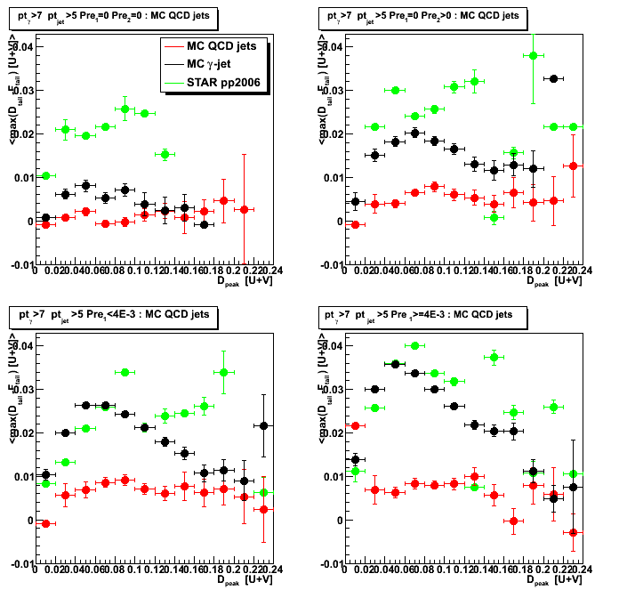
Figure 5: Mean < D_peak > vs. max(D_tail-F_tail) (profile on horisontal axis from Fig. 1)
For "no-preshower fired" case MC gamma-jet sample has a large average values than that from pp2006 data.
This reflects the same difference between pp2006 and MC gamma-jet sample at small D_peak values (see Fig. 2, upper left plot).
(Note: legend's color coding is wrong, colors scheme is the same as in Fig. 3)

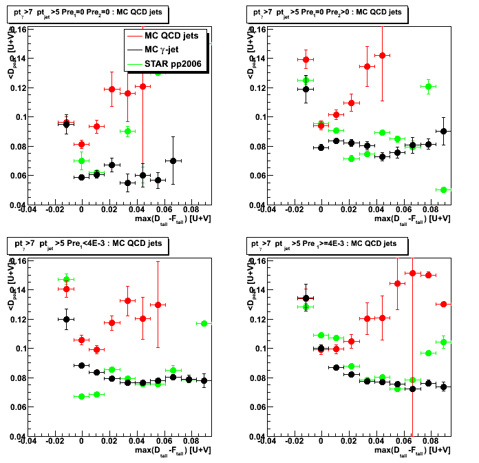
Figure 6: D_peak vs. gamma pt

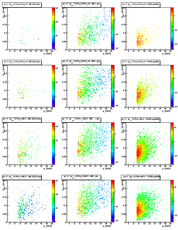
Figure 7: D_peak vs. gamma 3x3 tower cluster energy

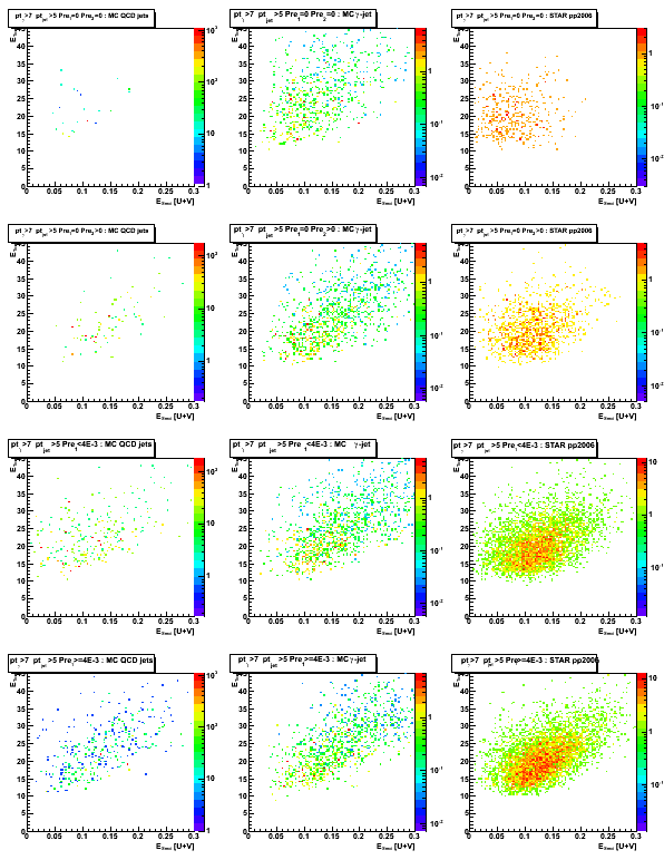
Figure 8: 3x3 cluster tower energy distribution

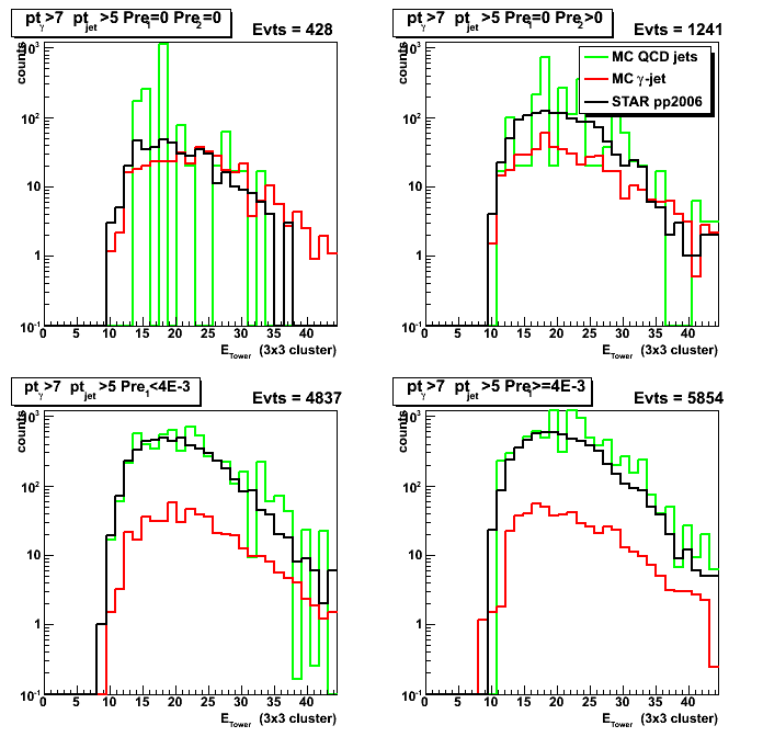
Figure 9: Gamma pt distribution

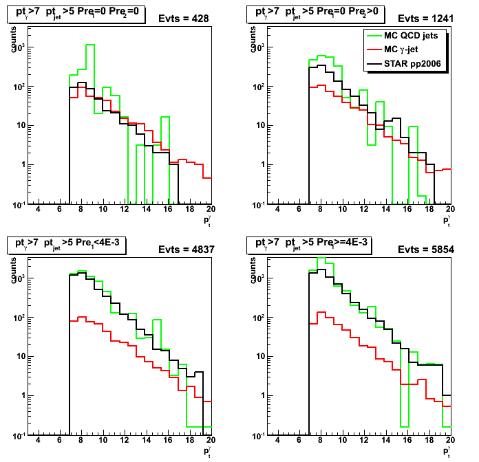
Signal/background separation

The simplest way to get signal/background separation is to draw a straight line
on sided residual plot (Fig. 1) in such a way that
it will contains most of the counts (signal) on the left side,
and use a distance to that line for both MC and pp2006 data samples
as a discriminant for signal/background separation.
To get the distance to the straight line one can rotate sided residual plot
by the angle which corresponds to the slope of this line,
and then project it on "rotated" max(D_tail-F_tail) axis.

Figure 10: Shows "rotated" sided residual plot by "5/6*(pi/2)" angle (this angle has been picked by eye).
One can see that now most of the counts for gamma-jet sample (middle column)
are on the left side from vertical axis.

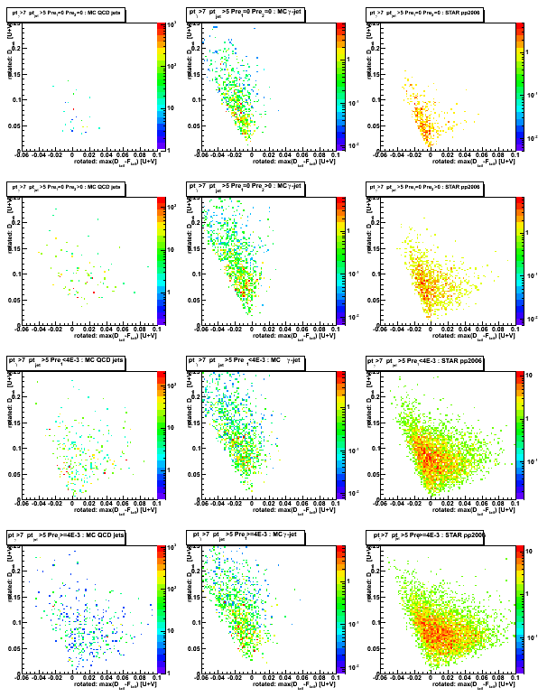
Figure 11: "Rotated" max(D_tail-F_tail) [projection on horizontal axis for Fig. 10]
Cut on "Rotated" max(D_tail-F_tail) can be used for signal/background separation.
From figure below one can see much better signal/background separation than in Fig. 3

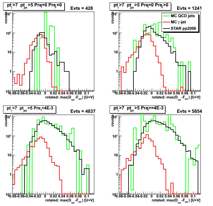
Figure 12: "Rotated" D_peak [projection on vertical axis for Fig. 10]

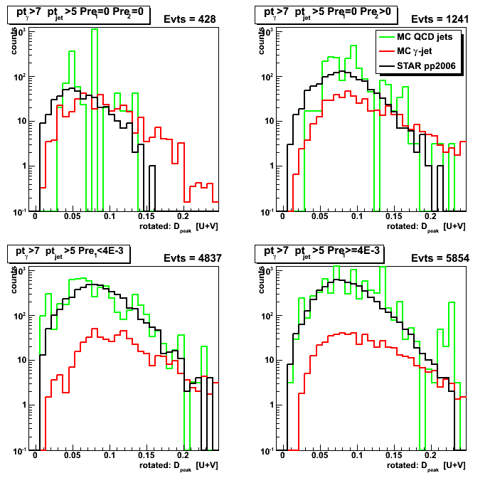
Optimizing the shape of s/bg separation line

Ideally, instead of straight line one needs to use
an actual shape of side residual distribution for MC gamma-jet sample.
This shape can be extracted and parametrized by the following procedure:

Get slices from sided residual plot for different D_peak values
From each slice get max(D_tail-F_tail) value
for which most of the counts appears on its left side (for example 80%),
Fit these set of points {D_peak slice, max(D_tail-F_tail)} with a polynomial function

The distance to that polynomial function can be used to determine our signal/background rejection efficiency.

This work is in progress...
Just last one figure showing shapes for 6 slices from sided plot.

Figure 13: max(D_tail-F_tail) for different slices in D_peak (scaled by the integral for each slice)

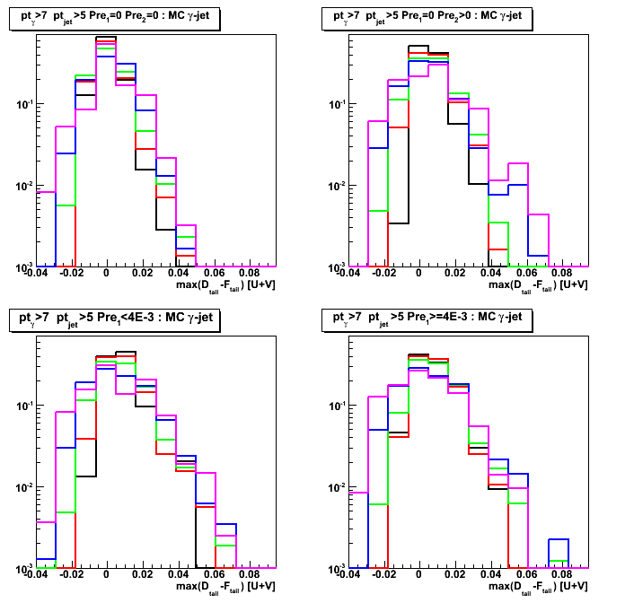
2008.09.30 Sided residual: purity, efficiency, and background rejection

Ilya Selyuzhenkov September 30, 2008

Data sets:

pp2006 - STAR 2006 pp longitudinal data (~ 3.164 pb^1)
after applying gamma-jet isolation cuts (note: R_cluster > 0.9 is used below).
gamma-jet - data-driven Pythia gamma-jet sample (~170K events). Partonic pt range 5-35 GeV.
QCD jets - data-driven Pythia QCD jets sample (~4M events). Partonic pt range 3-65 GeV.

Notations used in the plots:

Fit peak energy:
F_peak - integral within +-2 strips from maximum strip
Maximum strip determined by fitting procedure.
Float value converted ("cutted") to integer value.
Data peak energy:
D_peak - energy sum within +-2 strips from maximum strip (the same strip Id as for F_peak).
Data tails:
D_tail^left and D_tail^right.
Energy sum from 3rd strip up to 30 strips on the
left and right sides from maximum strip (excludes strips which contributes to D_peak)
Fit tails:
F_tail^left and F_tail^right.
Same definition as for D_tail, but integrals are calculated from a fit function.
Maximum sided residual:
max(D_tail-F_tail)
Maximum of the data minus fit energy on the left and right sides from the peak.

Determining cut line based on sided residual plot

Figure 1: Sided residual plot: D_peak vs. max(D_tail-F_tail)
Red lines show 4th order polynomial functions, a*x^4,
which have 80% of MC gamma-jet counts on the left side.
These lines are obtained independently for each of pre-shower condition
based on fit procedure shown in Fig. 3 below.

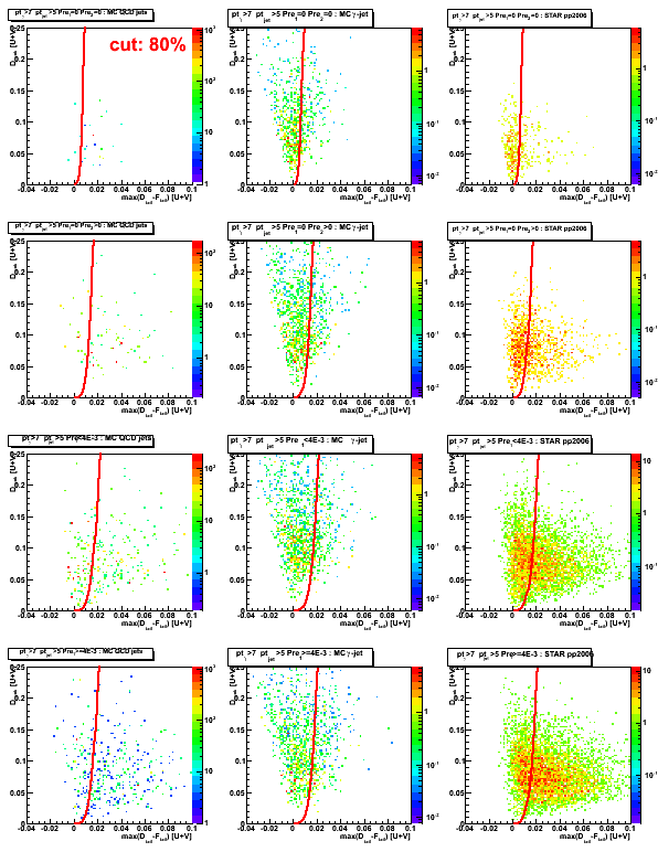
Figure 2: max(D_tail-F_tail) distribution
(projection on horizontal axis from sided residual plot, see Fig. 1 above)

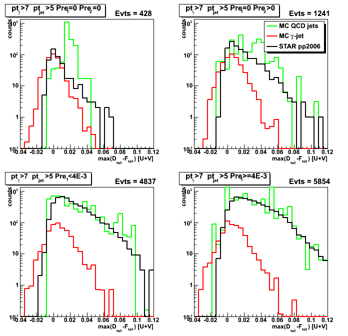
Figure 3: max(D_tail-F_tail) [at 80%] vs. D_peak.
For each slice (bin) in D_peak variable, the max(D_tail-F_tail) value
which has 80% of gamma-jet candidates on the left side are plotted.

Lines represent fits to MC gamma-jet points (shown in red) using different fit functions
(linear, 2nd, 4th order polynomials: see legend for color coding).
Note, that in this plot D_peak values are shown on horizontal axis.
Consequently, to get 2nd order polynomial fit on sided residual plot (Fig. 1),
one needs to use sqrt(D_peak) function.
The same apply to 4th order polynomial function.

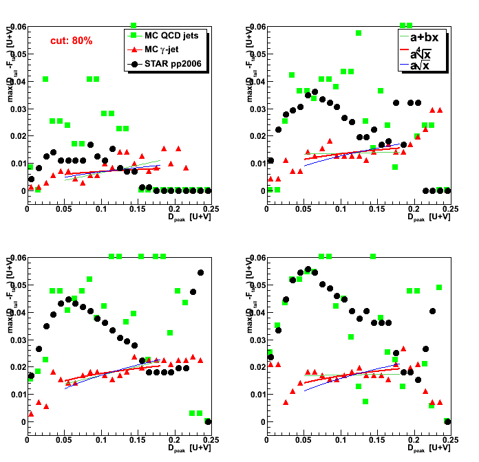
Figure 4: D_peak vs. horisontal distance from 4th order polinomial function to max(D_tail-F_tail) values.
(compare with Fig. 1: Now 80% of MC gamma-jet counts are on the left side from vertical axis)

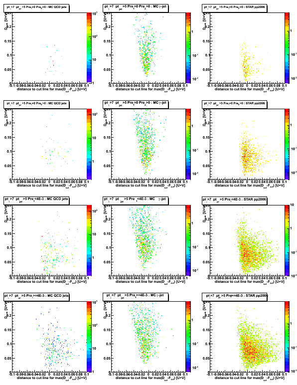
Figure 5: Horizontal distance from 4th order polynomial function to max(D_tail-F_tail)
[Projection on horizontal axis from Fig. 4]
Based on this plot one can obtain purity, efficiency, and rejection plots (see Fig. 6 below)

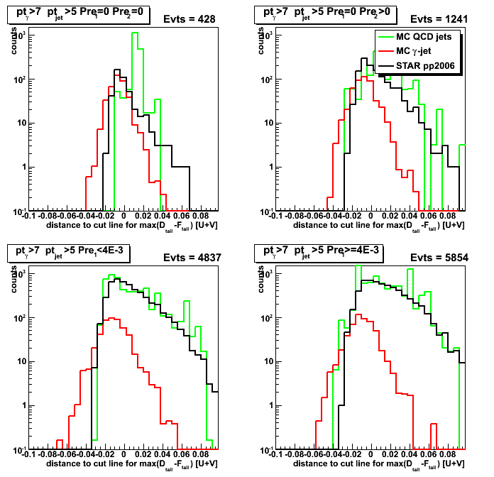
Gamma-jet purity, efficiency, and QCD background rejection

Horizontal distance plotted in Fig. 5 can be used as a cut
separating gamma-jet signal and QCD-jets background,
and for each value of this distance one can define
gamma-jet purity, efficiency, and QCD-background rejection:

gamma-jet purity is defined as the ratio of
the integral on the left for MC gamma-jet data sample, N[g-jet]_left,
to the sum of the integrals on the left for MC gamma-jet and QCD jets, N[QCD]_left, data samples:
Purity[gamma-jet] = N[g-jet]_left/(N[g-jet]_left+N[QCD]_left)
gamma-jet efficiency is defined as the ratio of
the integral on the left side for MC gamma-jet data sample, N[g-jet]_left,
to the total integral for MC gamma-jet data sample, N[g-jet]:
Efficiency[gamma-jet] = N[g-jet]_left/N[g-jet]
QCD background rejection is defined as the ratio of
the integral on the right side for MC QCD jets data sample, N[QCD]_right,
to the total integral for MC QCD jets data sample, N[QCD]:
Rejection[QCD] = N[QCD]_right/N[QCD]

Figure 6: Shows:
purity[g-jet] vs. efficiency[g-jet] (upper left);
rejection[QCD] vs. efficiency[g-jet] (upper right);
purity[g-jet] vs. rejection[QCD] (lower left);
pp2006 to MC ratio, N[pp2006]/(N[g-jet]+N[QCD]), vs. horizontal distance from Fig. 5 (lower right)

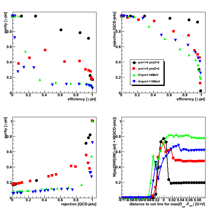
10 Oct

October 2008 posts

2008.10.13 Jet trees for Michael's gamma filtered events

Ilya Selyuzhenkov October 13, 2008

I have finished production of jet trees for Michael's gamma filtered events

You can find jet and skim file lists in my directory at IUCF disk (RCF):

Jet trees: /star/institutions/iucf/IlyaSelyuzhenkov/simu/JetTrees/JetTrees.list
Skim trees: /star/institutions/iucf/IlyaSelyuzhenkov/simu/JetTrees/SkimTrees.list
Log files: /star/institutions/iucf/IlyaSelyuzhenkov/simu/JetTrees/LogFiles.list

Number of jet events is 1284581 (1020 files).
Production size, including archived log files, is 4.0G.

The script to run jet finder:

/star/institutions/iucf/IlyaSelyuzhenkov/simu/JetTrees/20081008_gJet/StRoot/macros/RunJetSimuSkimFinder.C

JetFinder and JetMaker code:

/star/institutions/iucf/IlyaSelyuzhenkov/simu/JetTrees/20081008_gJet/StRoot/StJetFinder
/star/institutions/iucf/IlyaSelyuzhenkov/simu/JetTrees/20081008_gJet/StRoot/StJetMaker

For more details see these threads of discussions:

jetfinding list: thread 814
photon reconstruction list: thread 271 and thread 256

2008.10.14 Purity, efficiency, and background rejection: R_cluster > 0.98

Ilya Selyuzhenkov October 14, 2008

Data sets:

pp2006 - STAR 2006 pp longitudinal data (~ 3.164 pb^1)
after applying gamma-jet isolation cuts (note: R_cluster > 0.98 is used below).
gamma-jet - data-driven Pythia gamma-jet sample (~170K events). Partonic pt range 5-35 GeV.
QCD jets - data-driven Pythia QCD jets sample (~4M events). Partonic pt range 3-65 GeV.

Figure 1: Horizontal distance from 4th order polynomial function to max(D_tail-F_tail)
See this page for definition and more details

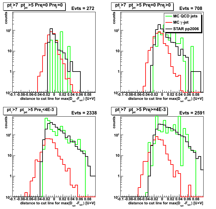
Figure 2:
purity[g-jet] vs. efficiency[g-jet] (upper left);
rejection[QCD] vs. efficiency[g-jet] (upper right);
purity[g-jet] vs. rejection[QCD] (lower left);
pp2006 to MC ratio, N[pp2006]/(N[g-jet]+N[QCD]), vs. horizontal distance (lower right)

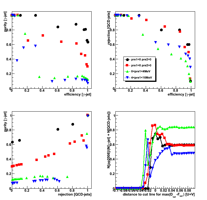
2008.10.15 Comparison of gamma-jets from Michael's filtered events vs. old MC samples

Ilya Selyuzhenkov October 15, 2008

Data sets:

pp2006 - STAR 2006 pp longitudinal data (~ 3.164 pb^1)
after applying gamma-jet isolation cuts (note: R_cluster > 0.9 is used below).
gamma-jet[gamma-filtered] - data-driven Prompt Photon [p6410EemcGammaFilter] events.
Partonic pt range 2-25 GeV.
QCD jets[gamma-filtered] - data-driven QCD [p6410EemcGammaFilter] events.
Partonic pt range 2-25 GeV.
gamma-jet [old] - data-driven Pythia gamma-jet sample (~170K events).
Partonic pt range 5-35 GeV.
Details on jet trees production for Michael's gamma filtered events can be found here.
QCD jets [old] - data-driven Pythia QCD jets sample (~4M events).
Partonic pt range 3-65 GeV.

Some observations:

Both Fig. 1a vs. Fig. 1b shows good statistics for old and new (gamma-filtered) MC gamma-jet samples
Fig. 1c shows poor statistics for QCD background sample
within partonic pt range 5-10GeV (only 3 counts for "pre1=0 & pre2=0" condition).
Fig. 1d (new QCD sample) has much more counts in the same region,
but it is still only 20-25 entries for the case when
none of EEMC pre-shower layers fired (upper left corner - our purest gamma-jet sample).
This may be still insufficient for a various cuts systematic study.
Fig. 2 and Fig. 3 shows nice agreement between data and MC
for both old and new (gamma-filtered) MC samples.
For pre-shower1>0 case this agreement persists across full range of gamma's pt (7GeV and above).
Upper plots in Fig. 3 shows some difference between data and Monte-Carlo,
what could be effect from l2gamma trigger,
which has not been yet applied for MC events.

Figure 1a: partonic pt for gamma-jet [old] events
after analysis cuts and partonic pt bin weighting
(Note:Arbitrary absolute scale)

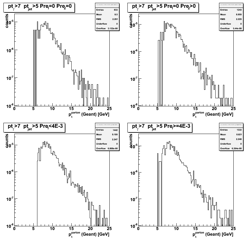
Figure 1b: partonic pt for gamma-jet [gamma-filtered] events after analysis cuts.
Michael's StBetaWeightCalculator has been used to caclulate partonic pt weights

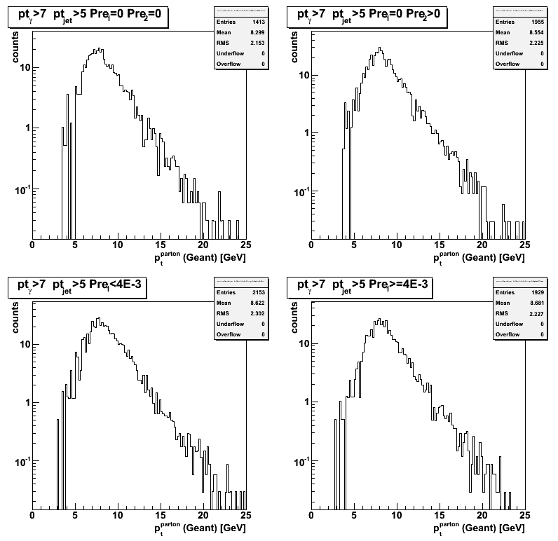
Figure 1c: partonic pt for QCD jets [old] events
after analysis cuts and partonic pt bin weighting
(Note:Arbitrary absolute scale)

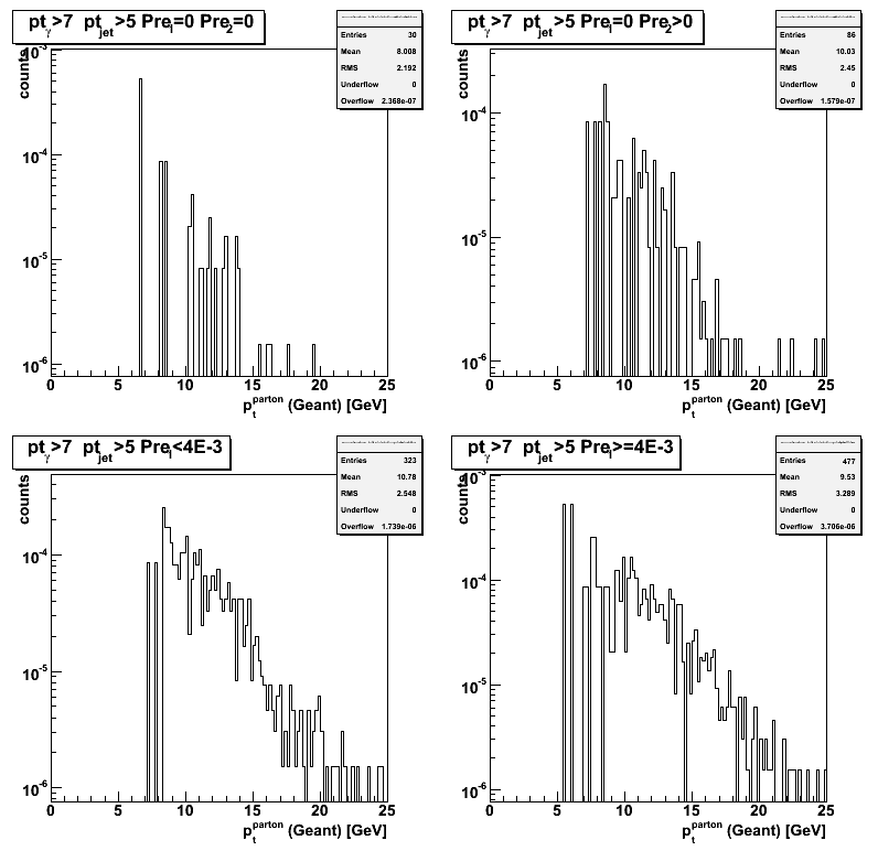
Figure 1d: partonic pt for QCD jets [gamma-filtered] events after analysis cuts.
Michael's StBetaWeightCalculator has been used to caclulate partonic pt weights

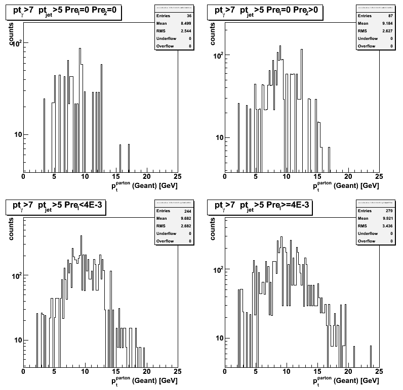
Figure 2: reconstructed gamma pt: old MC vs. pp2006 data (scaled to the same luminosity)

Figure 3: reconstructed gamma pt: gamma-filtered MC vs. pp2006 data (scaled to the same luminosity)

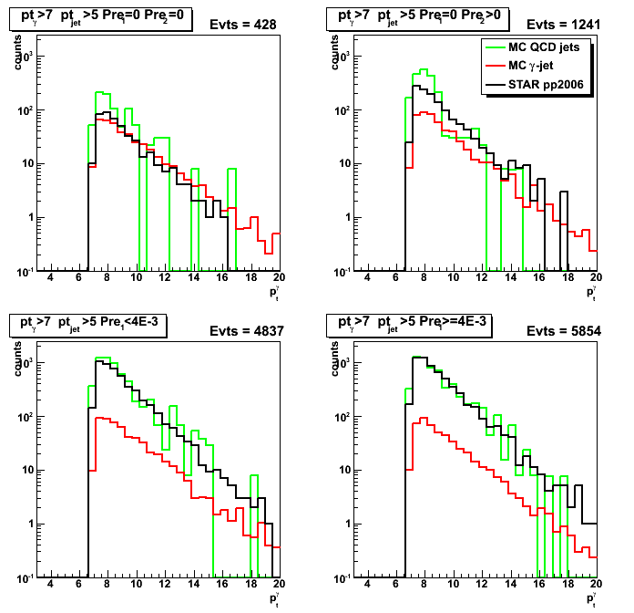
2008.10.15 Purity vs. efficiency from gamma-filtered events: R_cluster > 0.9 vs. R_cluster > 0.98

Ilya Selyuzhenkov October 15, 2008

Data sets:

pp2006 - STAR 2006 pp longitudinal data (~ 3.164 pb^1)
after applying gamma-jet isolation cuts (note: R_cluster > 0.9 or > 0.98 is used below).
gamma-jet[gamma-filtered] - data-driven Prompt Photon [p6410EemcGammaFilter] events.
Partonic pt range 2-25 GeV.
QCD jets[gamma-filtered] - data-driven QCD [p6410EemcGammaFilter] events.
Partonic pt range 2-25 GeV.

Gamma-jet candidates from MC gamma filtered events: R_cluster > 0.9

Figure 1: Horizontal distance from sided residual plot: R_cluster > 0.9
(see Figs. 1-5 from this post for horizontal distance definition)

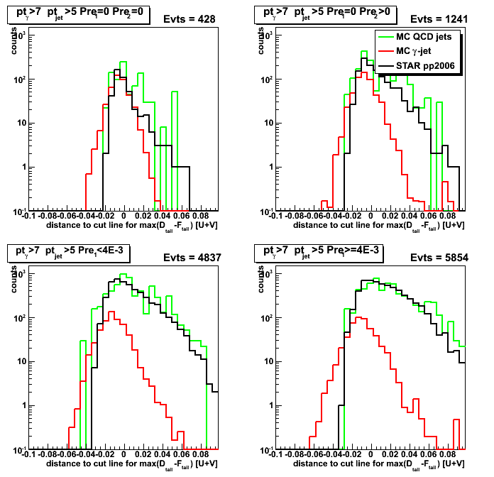
Figure 2: Purity/efficiency/rejection, and data to MC[gamma-jet+QCD] ratio plots: R_cluster > 0.9
(see text above Fig. 6 from this post for purity, efficiency, and background rejection definition)

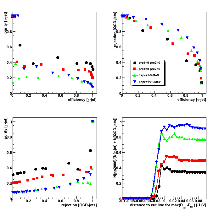
Gamma-jet candidates from MC gamma filtered events: R_cluster > 0.98

Figure 3: Reconstructed gamma pt: R_cluster > 0.98

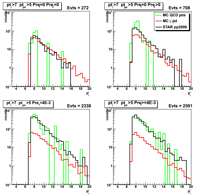
Figure 4: Horizontal distance from sided residual plot: R_cluster > 0.98

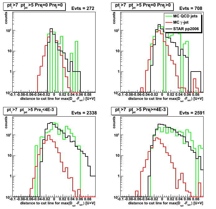
Figure 5: Purity/efficiency/rejection, and data to MC[gamma-jet+QCD] ratio plots: R_cluster > 0.98

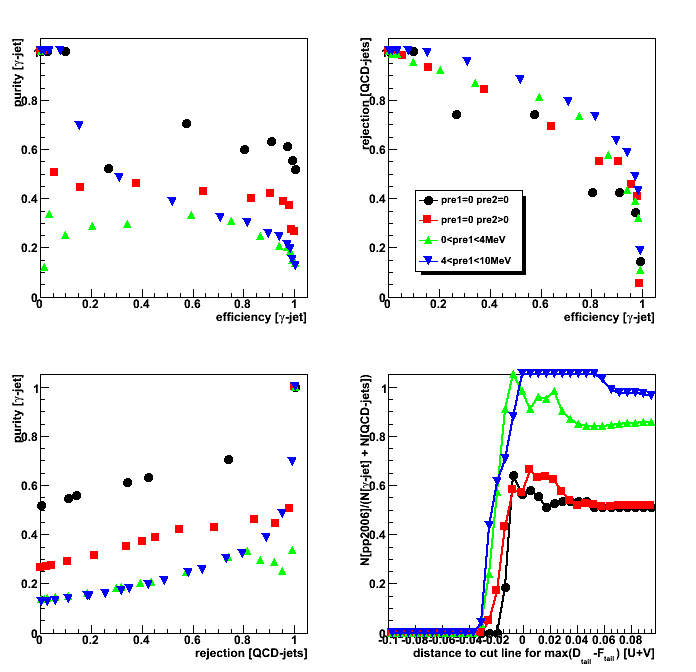
2008.10.21 Shower shapes, 5/25 strips cluster energy, raw vs. data-driven MC

Ilya Selyuzhenkov October 21, 2008

Data sets:

pp2006 - STAR 2006 pp longitudinal data (~ 3.164 pb^1)
after applying gamma-jet isolation cuts (R_cluster > 0.9 is used below).
gamma-jet[gamma-filtered] - data-driven Prompt Photon [p6410EemcGammaFilter] events.
Partonic pt range 2-25 GeV.
QCD jets[gamma-filtered] - data-driven QCD [p6410EemcGammaFilter] events.
Partonic pt range 2-25 GeV.

Some comments:

Overall comment: effect of data-driven shower shape replacement procedure
on QCD background events is small, except probably pre1=0 pre2=0 case.
Fig. 1-3, upper left plots (pre1=0 pre2=0) show that
average energy per strip in data-driven gamma-jet MC (i.e. solid red square in Fig. 3)
is systematically higher than that for pp2006 data (black circles in Fig. 3).

Note, that there is an agreement between SMD shower shapes
for pp2006 data and data-driven gamma-jet simulations
if one scales them to the same peak value
(Compare red vs. black in upper left plot from Fig. 1 at this link)
Fig. 4, upper left plot (pre1=0 pre2=0):
Integrated SMD energy from 25 strips
in raw gamma-jet simulations (red line) match pp2006 data (black line)
in the region where signal to background ratio is high, E_smd(25-strips)>0.1GeV.
This indicates that raw MC does a good job in
reproducing total energy deposited by direct photon.
Fig. 5, upper left plot (pre1=0 pre2=0):
There is mismatch between distributions of energy in 25 strips cluster
from data-driven gamma-jet simulations and pp2006 data.
This probably reflects the way we scale our library shower shapes
in data-driven shower shape replacement procedure.
Currently, the scaling factor for the library shape is calculated based on the ratio
of direct photon energy from Geant record to the energy of the library photon.
Our library is build out of photons from eta-meson decay,
which has been reconstructed by running pi0 finder.
The purity of the library is about 70% (see Fig. 1 at this post for more details).

The improvement of scaling procedure could be to
preserve total SMD energy deposited within 25 strips from raw MC,
and use that energy to scale shower shapes from the library.
Fig. 6, upper left plot (pre1=0 pre2=0):
Mismatch between integrated 5-strip energy for raw MC and pp2006 in Fig. 6
corresponds to "known" difference in shower shapes from raw Monte-Carlo and real data.

Figure 1: SMD shower shapes: data, raw, and data-driven MC (40 strips).
Vertical axis shows average energy per strip (no overall shower shapes scaling)

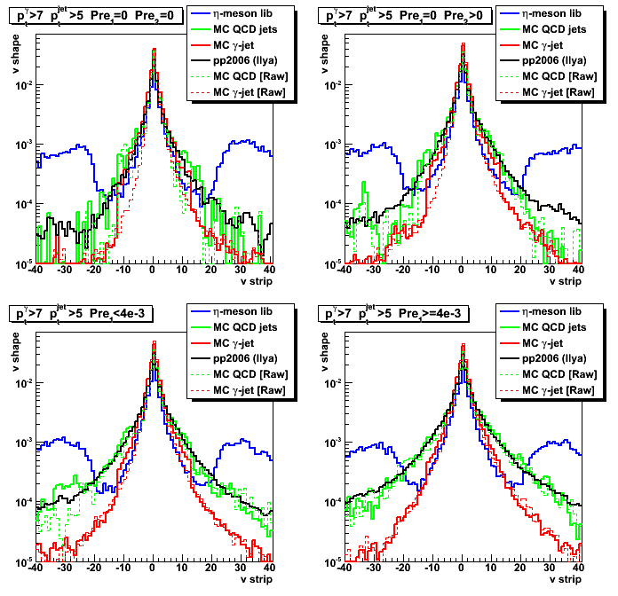
Figure 2: Shower shapes: data, raw, and data-driven MC (12 strips)

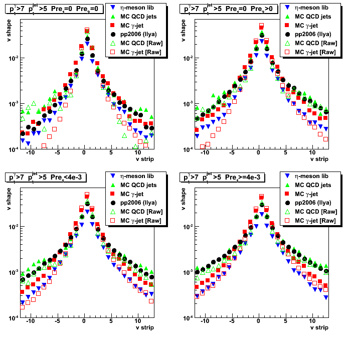
Figure 3: Shower shapes: data, raw, and data-driven MC (5 strips)

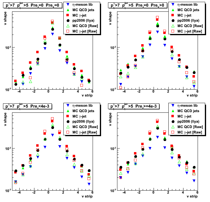
Figure 4: 25 strips SMD cluster energy for raw Monte-Carlo
(Note: type in x-axis lables, should be "25 strip peak" instead of 5)

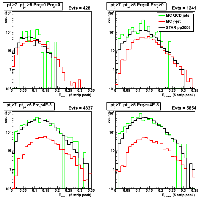
Figure 5: 25 strips SMD cluster energy for data-driven Monte-Carlo

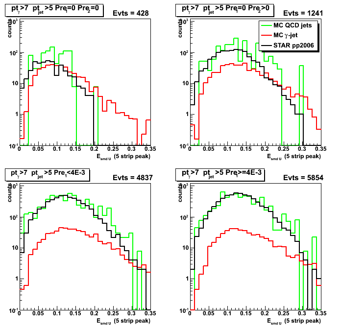
Figure 6: 5 strips SMD peak energy for raw Monte-Carlo

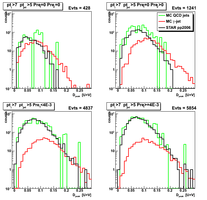
Figure 7: 5 strips SMD peak energy for data-driven Monte-Carlo

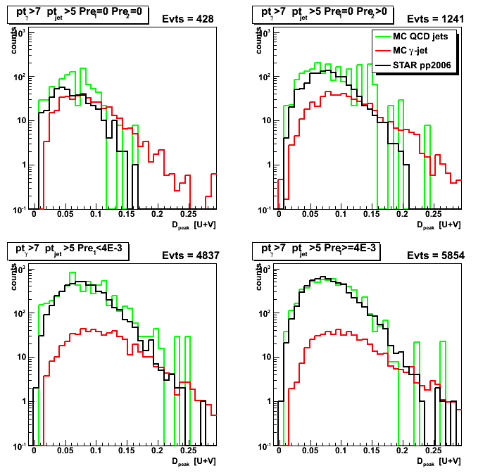
Figure 8:Energy from the right tail (up to 30 strips) for raw Monte-Carlo

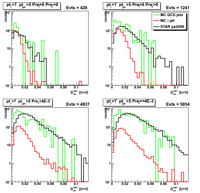
Figure 9:Energy from the right tail (up to 30 strips) for data-driven Monte-Carlo

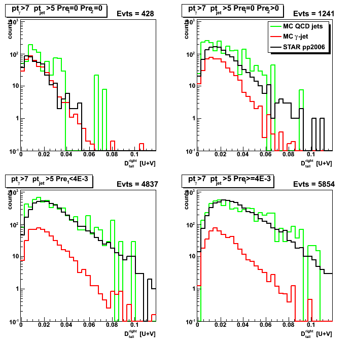
2008.10.27 SMD-based shower shape scaling: 25 strips cluster energy, raw vs. data-driven MC

Ilya Selyuzhenkov October 27, 2008

Data sets:

pp2006 - STAR 2006 pp longitudinal data (~ 3.164 pb^1)
after applying gamma-jet isolation cuts (R_cluster > 0.9 is used below).
gamma-jet[gamma-filtered] - data-driven Prompt Photon [p6410EemcGammaFilter] events.
Partonic pt range 2-25 GeV.
QCD jets[gamma-filtered] - data-driven QCD [p6410EemcGammaFilter] events.
Partonic pt range 2-25 GeV.

Shower shapes scaling options in data-driven maker:

scale = E_smd^geant / E_smd^library (default)
E_smd^geant is SMD energy associated with given photon
integrated over +/- 12 strips from raw Monte-Carlo,
and E_smd^library is SMD energy from +/- 12 strips for the library photon.
scale = E_Geant / E_library (used before in all posts)
E_Geant is thrown photon energy from Geant record,
and E_library is stand for energy of the library photon.

In all figures below (exept for pp2006 data and raw Monte-Carlo)
the SMD based shower shape scaling has been used.

Figure 1: SMD shower shapes: data, raw, and data-driven MC (40 strips).
Vertical axis shows average energy per strip (no overall shower shapes scaling)

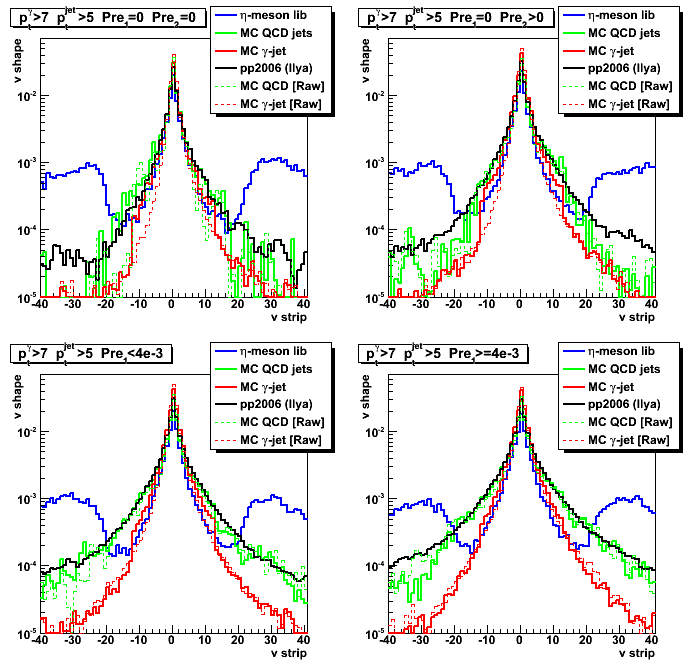
Figure 2: Shower shapes: data, raw, and data-driven MC (12 strips)

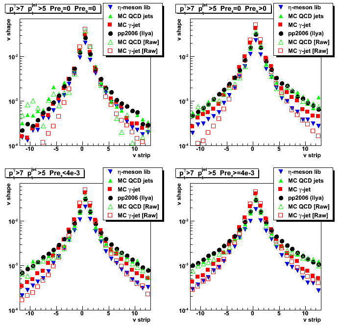
Figure 3: Shower shapes: data, raw, and data-driven MC (5 strips)

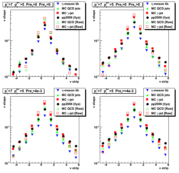
Figure 4: 25 strips SMD cluster energy for data-driven Monte-Carlo
(SMD based shower shape scaling)

Figure 5: 25 strips SMD cluster energy for raw Monte-Carlo
Note, the difference between results in Fig. 4 and 5. for MC gamma-jets (shown in red)
at low energy (Esmd < 0.04) for pre1=0 pre2=0 case.
This effect is due to the "Number of strips fired in 5-strips cluster > 3" cut.
In data-driven Monte-Carlo we may have shower shapes
with small number of strips fired (rejected in raw Monte-Carlo)
to be replaced by library shape with different (bigger) number of strips fired.
This mostly affects photons which starts to shower
later in the detector and only fires few strips (pre1=0 pre2=0 case)

2008.10.30 Various cuts study (pt, Esmd, 8 strips replaced)

Ilya Selyuzhenkov October 30, 2008

Below are links to drupal pages
with various SMD energy distributions and shower shapes
for the following set of cuts/conditions:

Case A: pt > 7 GeV, +/- 12 strips replaced
Case B: pt > 7 GeV, +/- 8 strips replaced
Case C: pt > 7 GeV, +/- 12 strips replaced, E_smd(25strips) > 0.1
Case D: pt > 8.5 GeV, +/- 12 strips replaced

2008.10.30 Distance to cut line from sided residual

Figure 1: Case A

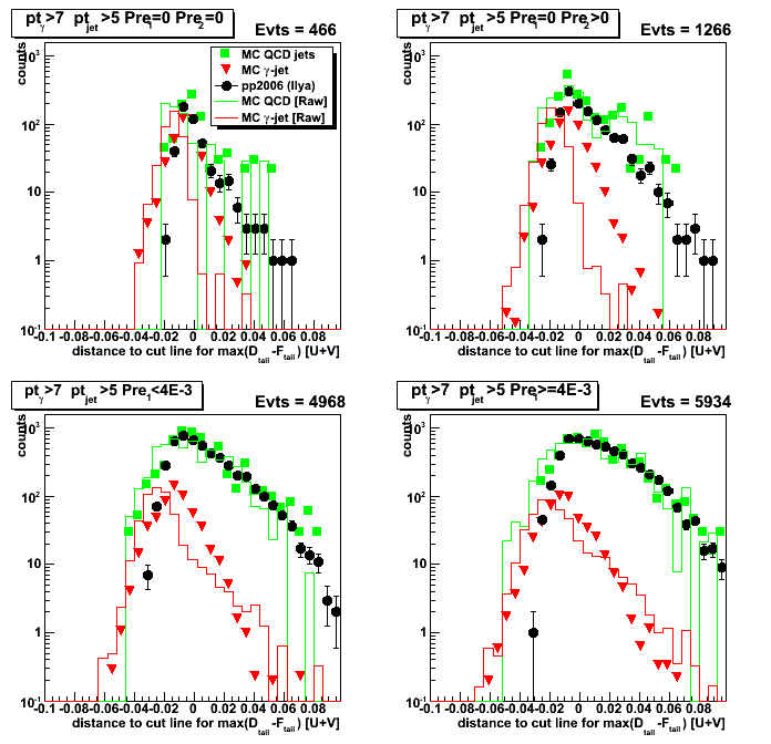
Figure 2:Case B

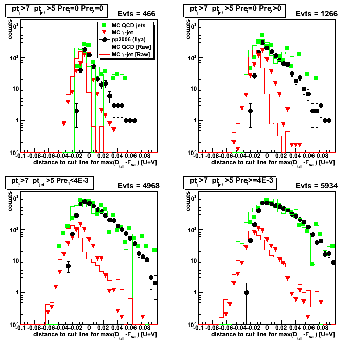
Figure 3:Case C

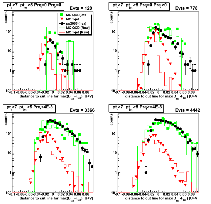
Figure 4:Case D

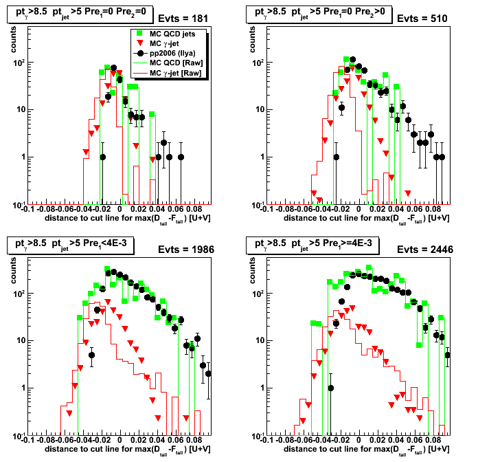
2008.10.30 SMD shower shapes: data, raw, and data-driven MC (12 strips)

Figure 1: Case A

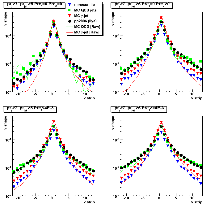
Figure 2:Case B

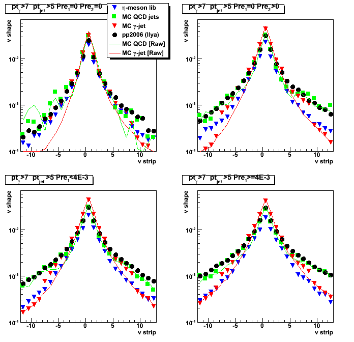
Figure 3:Case C

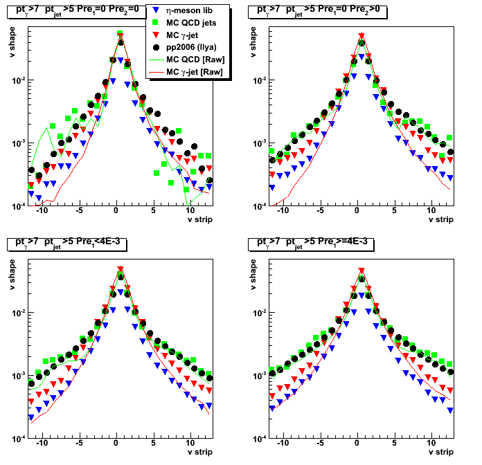
Figure 4:Case D

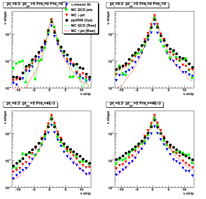
2008.10.30 SMD shower shapes: data, raw, and data-driven MC (30 strips)

Figure 1: Case A

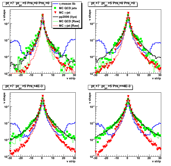
Figure 2: Case B

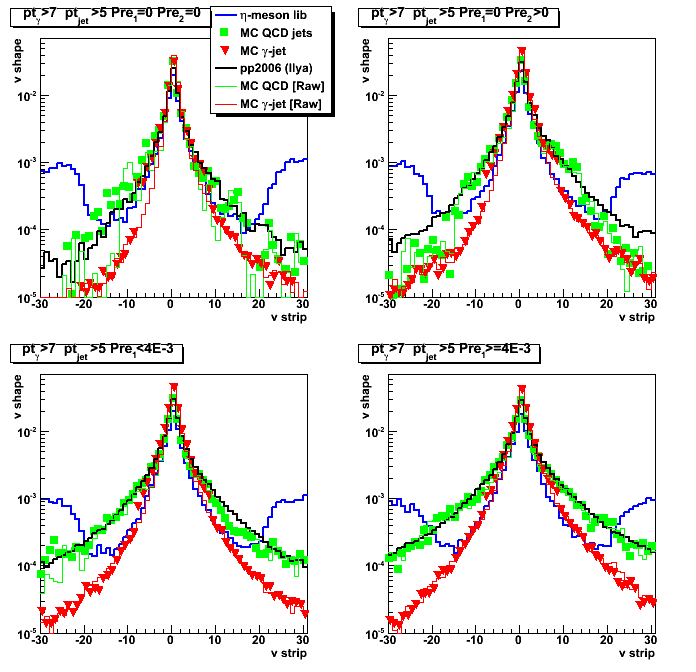
Figure 3: Case C

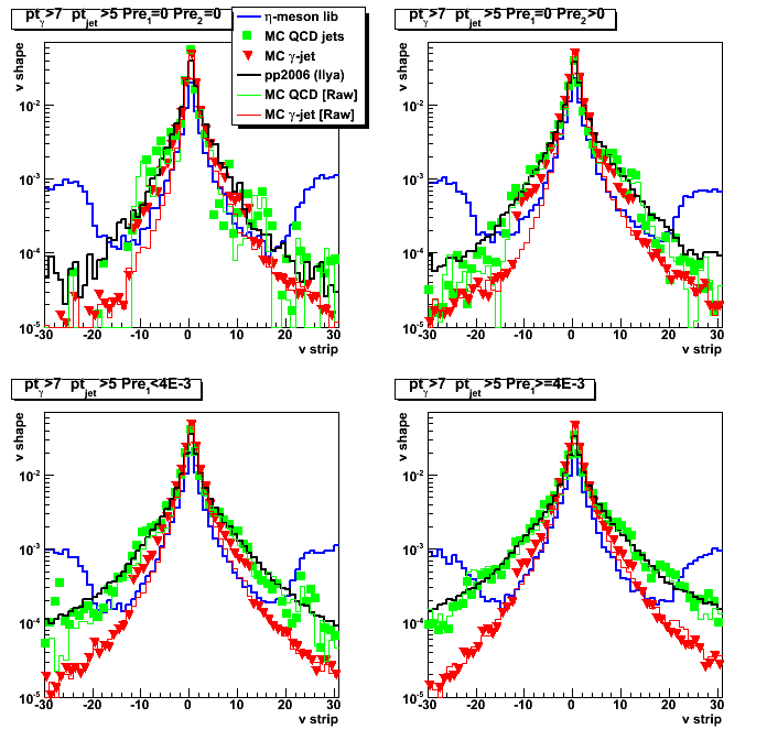
Figure 4: Case D

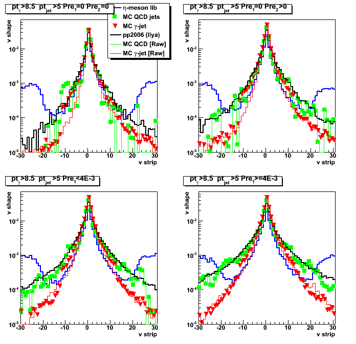
2008.10.30 Sided residual

Figure 1: Case A

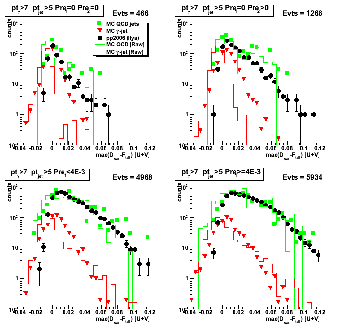
Figure 2:Case B

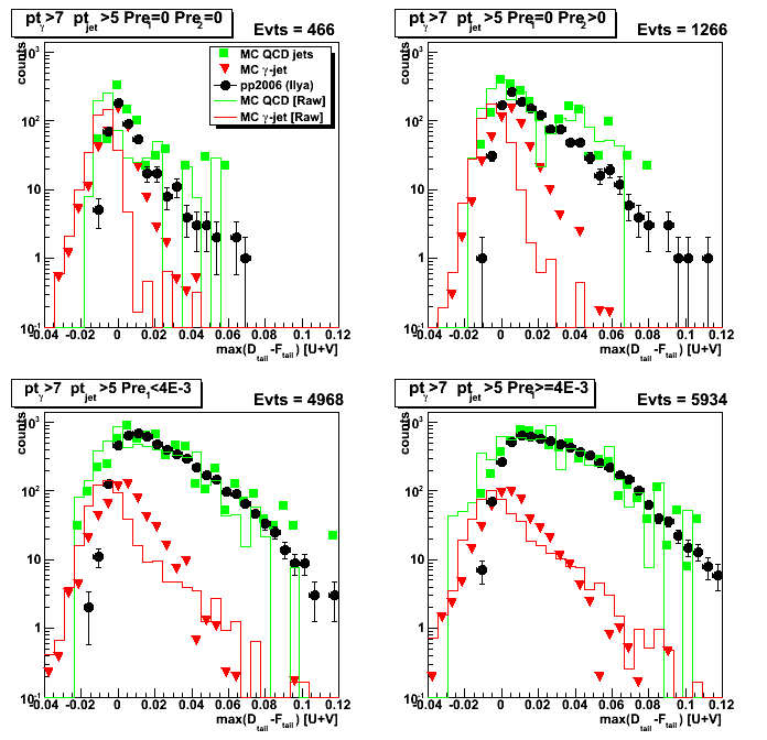
Figure 3:Case C

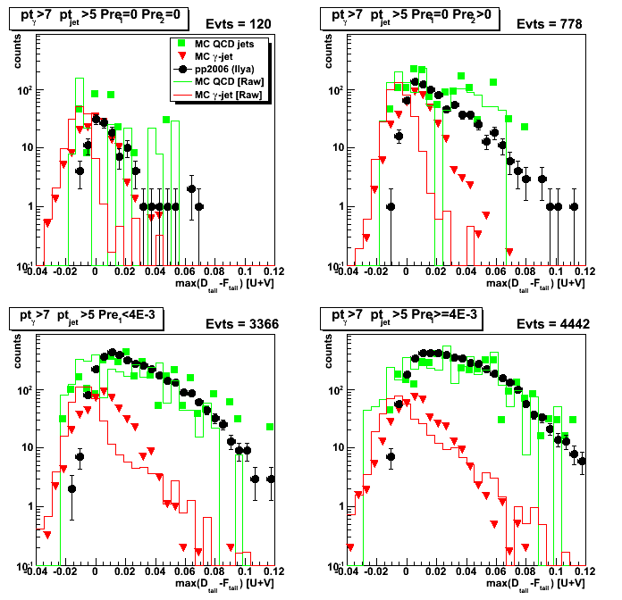
Figure 4:Case D

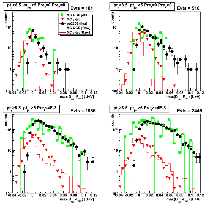
2008.10.30 Smd emergy for left tail (-3 to -30 strips)

Figure 1: Case A

Figure 2:Case B

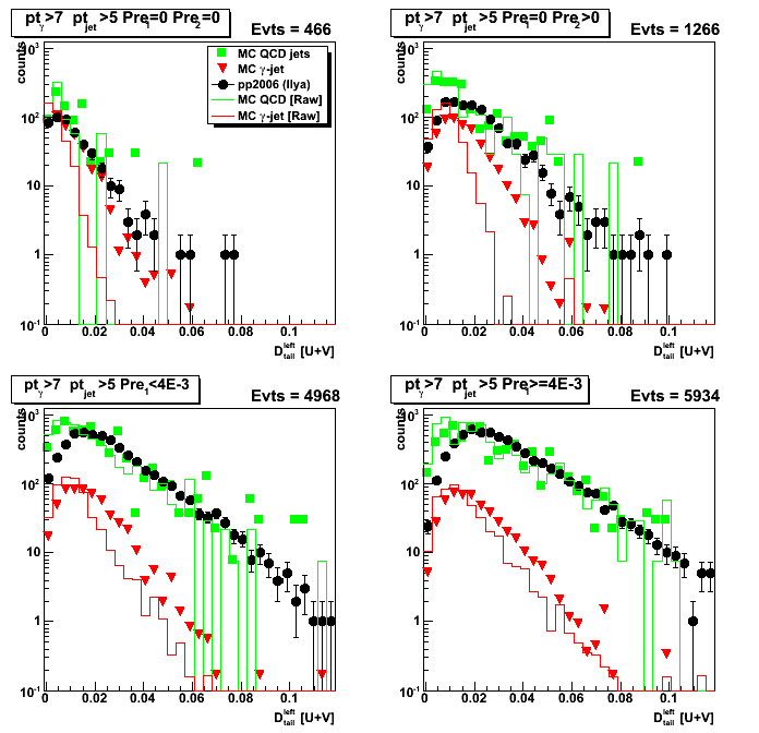
Figure 3:Case C

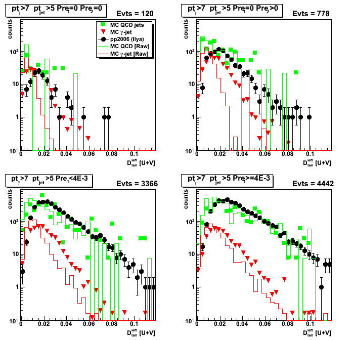
Figure 4:Case D

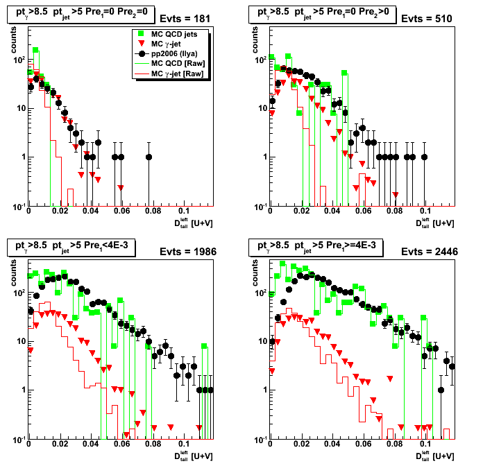
2008.10.30 Smd emergy for right tail (3 to 30 strips)

Figure 1: Case A

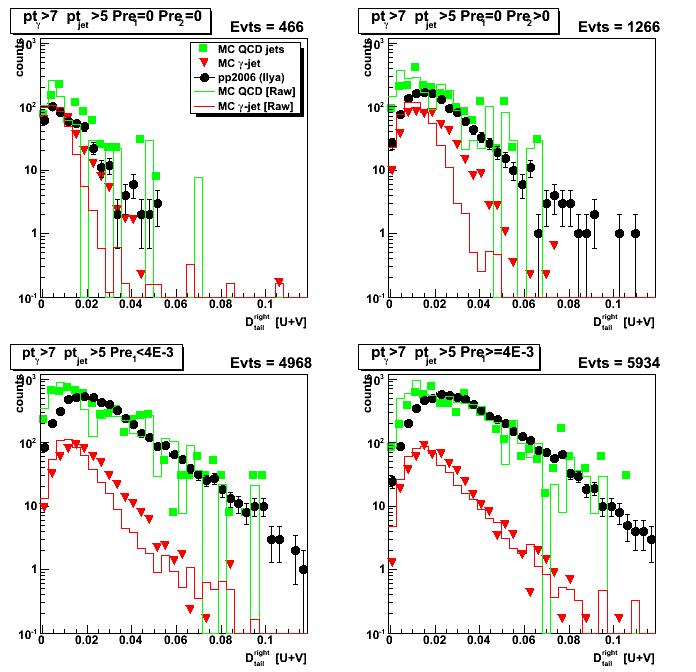
Figure 2:Case B

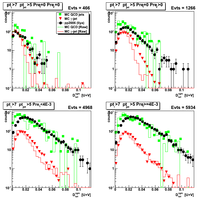
Figure 3:Case C

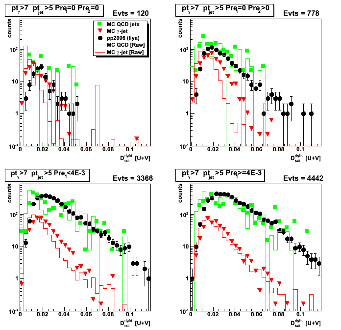
Figure 4:Case D

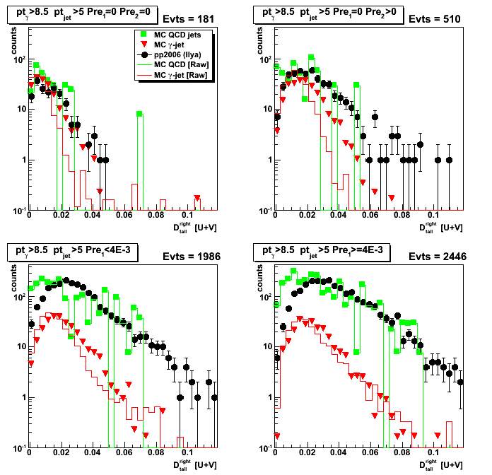
2008.10.30 Smd energy for 25 central strips

Figure 1: Case A

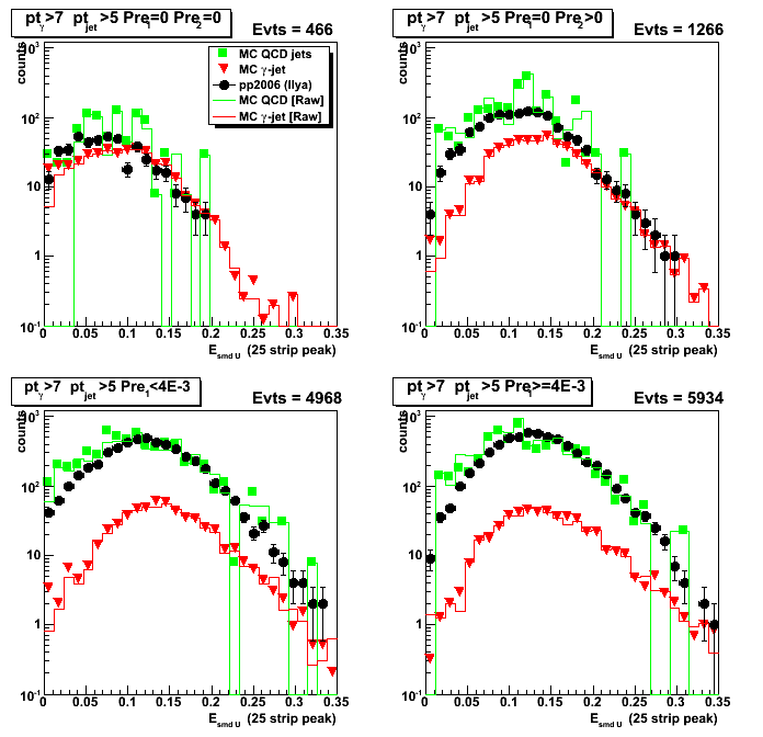
Figure 2:Case B

Figure 3:Case C

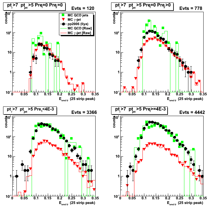
Figure 4:Case D

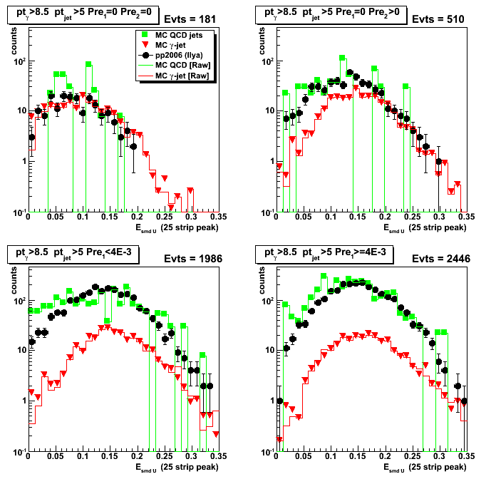
2008.10.30 Smd energy for 5 central strips

Figure 1: Case A

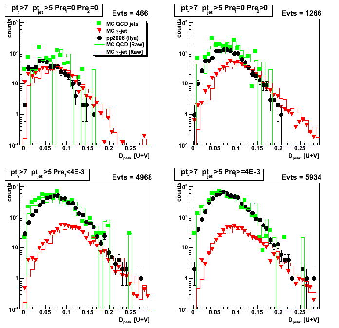
Figure 2:Case B

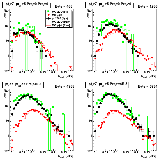
Figure 3:Case C

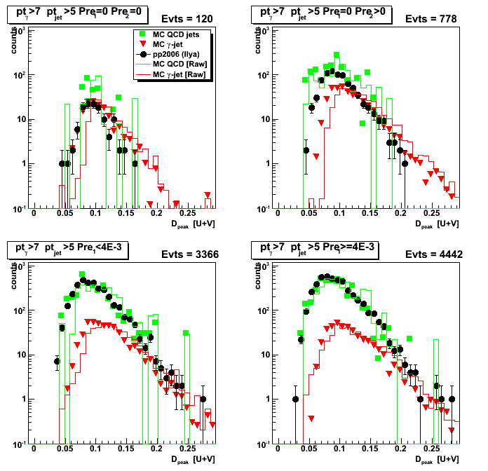
Figure 4:Case D

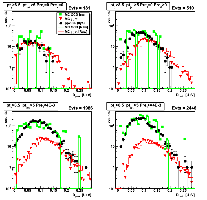
11 Nov

November 2008 posts

2008.11.06 Gamma-jet reconstruction with the Endcap EMC (Analysis status update)

Ilya Selyuzhenkov November 06, 2008

Gamma-jet reconstruction with the Endcap EMC (Analysis status update for Spin PWG)

latest version (pdf)
Version 3: pdf or odp (for spin PWG)
Version 2: pdf or odp (after phana comments)
Version 1: pdf or odp (draft for phana meeting)

2008.11.11 Yields vs. analysis cuts

Ilya Selyuzhenkov November 11, 2008

Data sets:

pp2006 - STAR 2006 pp longitudinal data (~ 3.164 pb^1)
after applying gamma-jet isolation cuts (R_cluster > 0.9 is used below).
gamma-jet[gamma-filtered] - data-driven Prompt Photon [p6410EemcGammaFilter] events.
Partonic pt range 2-25 GeV.
QCD jets[gamma-filtered] - data-driven QCD [p6410EemcGammaFilter] events.
Partonic pt range 2-25 GeV.

Figure 1: Reconstructed gamma pt for di-jet events and
Geant cuts: pt_gamma[Geant] > 7GeV and 1.05 < eta_gamma[Geant] < 2.0
Total integral for the histogram is: N_total = 5284
(after weighting different partonic pt bins and scaled to 3.164pb^-1).
Compare with number from Jim Sowinski study for
Endcap East+West gamma-jet and pt>7 GeV: N_Jim = 5472
( Jim's numbers are scaled to 3.164pb^-1 : [2539+5936]*3.164/4.9)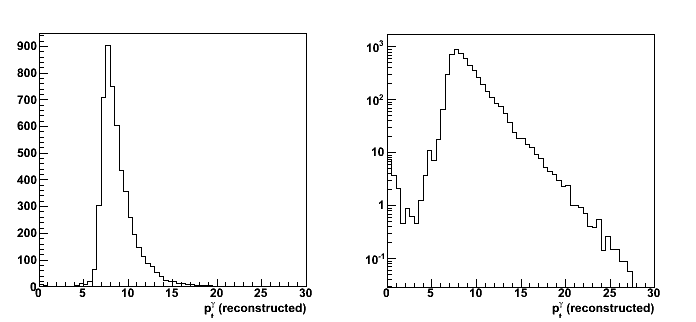

Figure 2: Reconstructed jet pt for di-jet events and the same cuts as in Fig. 1

Yield vs. various analysis cuts

List of cuts (sorted by bin number in Figs. 2 and 3):

N_events : total number of di-jet events found by the jet-finder
cos(phi_gamma - phi_jet) < -0.8 : gamma-jet opposite in phi
R_{3x3cluster} > 0.9 : Energy in 3x3 cluster of EEMC tower to the total jet energy
R_EM^jet < 0.9 : neutral energy fraction cut for on away side jet
N_ch=0 : no charge tracks associated with a gamma candidate
N_bTow = 0 : no barrel towers associated with a gamma candidate (gamma in the endcap)
N_(5-strip cluster)^u > 2 : minimum number of strips in EEMC SMD u-plane cluster around peak
N_(5-strip cluster)^v > 2 : minimum number of strips in EEMC SMD v-plane cluster around peak
gamma-algo fail : my algorithm failed to match tower with SMD uv-intersection, etc...
Tow:SMD match : SMD uv-intersection has a tower which is not in a 3x3 cluster

Figure 3: Number of accepted events vs. various analysis cuts
The starting number of events (shown in first bin of the plots) is
the number of di-jets with reconstructed gamma_pt>7 GeV and jet_pt>5 GeV
upper left: cuts applied independently
upper right: cuts applied sequentially
lower left: ratio of pp2006 data vs. MC sum of gamma-jet and QCD-jets events (cuts applied independently)
lower right:ratio of pp2006 data vs. MC sum of gamma-jet and QCD jets events (cuts applied sequentially)

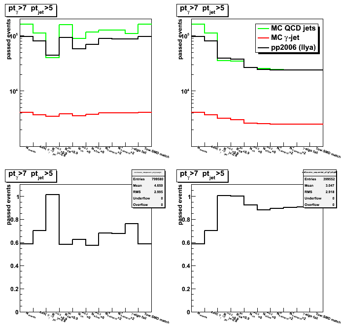
Figure 4: Number of accepted events vs. various analysis cuts
Data from Fig. 3 (upper plots) scaled to the initial number of events from first bin:
left: cuts applied independently
right: cuts applied sequentially

2008.11.18 Cluster isolation cuts: 2x1 vs. 2x2 vs. 3x3

Ilya Selyuzhenkov November 18, 2008

Data sets:

pp2006 - STAR 2006 pp longitudinal data (~ 3.164 pb^1)
after applying gamma-jet isolation cuts (no R_cluster cut applied for this study).
gamma-jet[gamma-filtered] - data-driven Prompt Photon [p6410EemcGammaFilter] events.
Partonic pt range 2-25 GeV.
QCD jets[gamma-filtered] - data-driven QCD [p6410EemcGammaFilter] events.
Partonic pt range 2-25 GeV.

2x1, 2x2, and 3x3 clusters definition:

3x3 cluster: tower energy sum for 3x3 patch around highest tower
2x2 cluster: tower energy sum for 2x2 patch
which are closest to 3x3 tower patch centroid.
3x3 tower patch centroid is defined based
on tower energies weighted wrt tower centers:
centroid = sum{E_tow * r_tow} / sum{E_tow}.
Here r_tow=(x_tow, y_tow) denotes tower center.
2x1 cluster: tower energy sum for high tower plus second highest tower in 3x3 patch
r=0.7 energy is calculated based on towers
within a radius of 0.7 (in delta phi and eta) from high tower

Cuts applied

all gamma-jet candidate selection cuts except 3x3/r=0.7 energy isolation cut

Results for 2x1, 2x2, and 3x3 clusters

Energy fraction in NxN cluster in r=0.7 radius
2x1, 2x2, 3x3 patch to jet radius of 0.7 energy ratios
Yield vs. NxN cluster energy fraction in r=0.7
For a given cluster energy fraction yield is defined as an integral on the right
Efficiency vs. NxN cluster energy fraction in r=0.7
For a given cluster energy fraction
efficiency is defined as the yield (on the right)
normalized by the total integral (total yield)

Efficiency vs. NxN cluster energy fraction in r=0.7

Figure 1b: 2x1/0.7 ratio

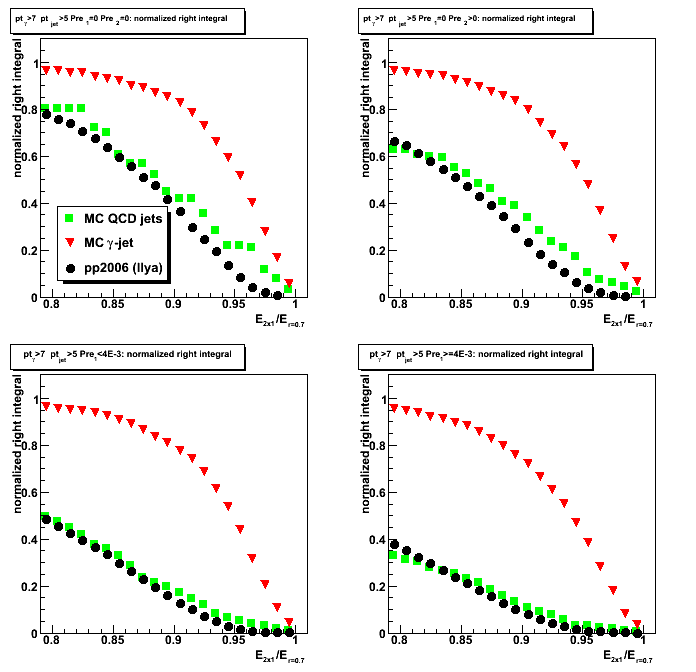
Figure 2b: 2x2/0.7 ratio

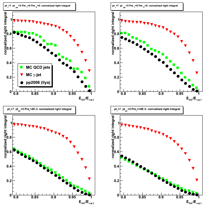
Figure 3b: 3x3/0.7 ratio

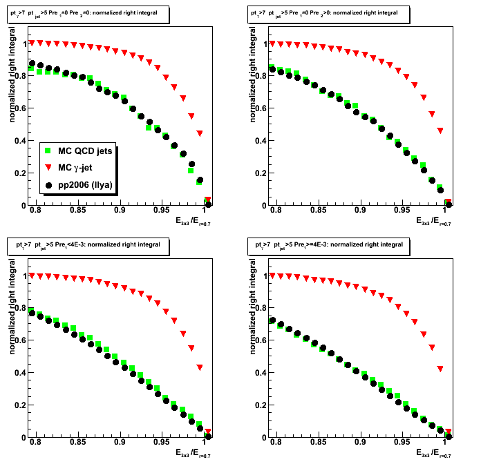
Figure 4b: 3x3/0.7 ratio but only using towers which passed jet finder threshold

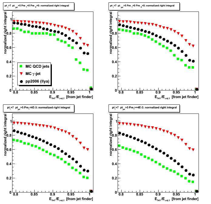
Energy fraction in NxN cluster within r=0.7 radius

Figure 1a: 2x1/0.7 ratio

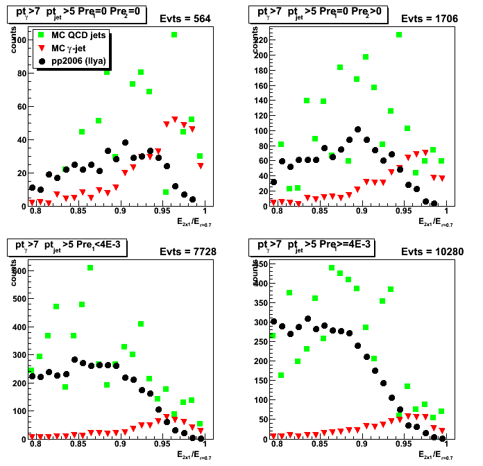
Figure 2a: 2x2/0.7 ratio

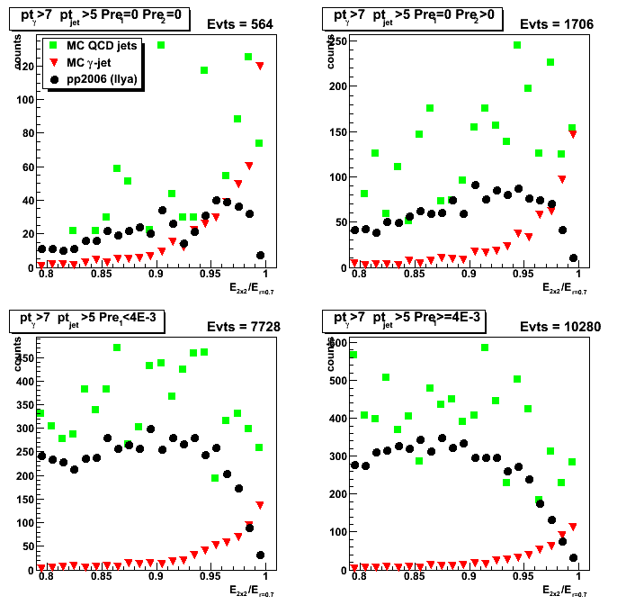
Figure 3a: 3x3/0.7 ratio

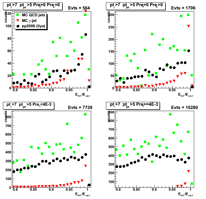
Figure 4a: 3x3/0.7 ratio but only using towers which passed jet finder threshold

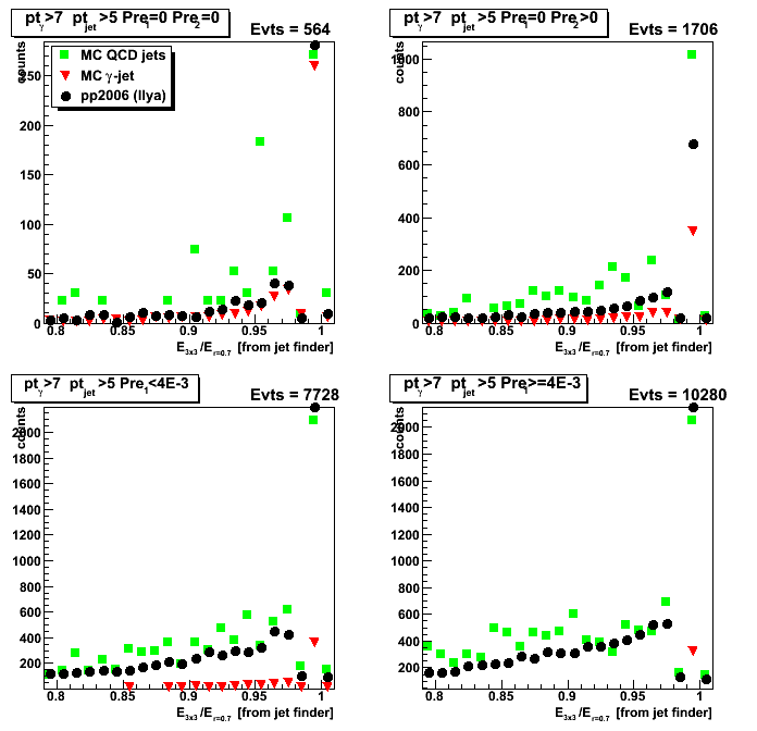
Yield vs. NxN cluster energy fraction in r=0.7

Figure 1c: 2x1/0.7 ratio

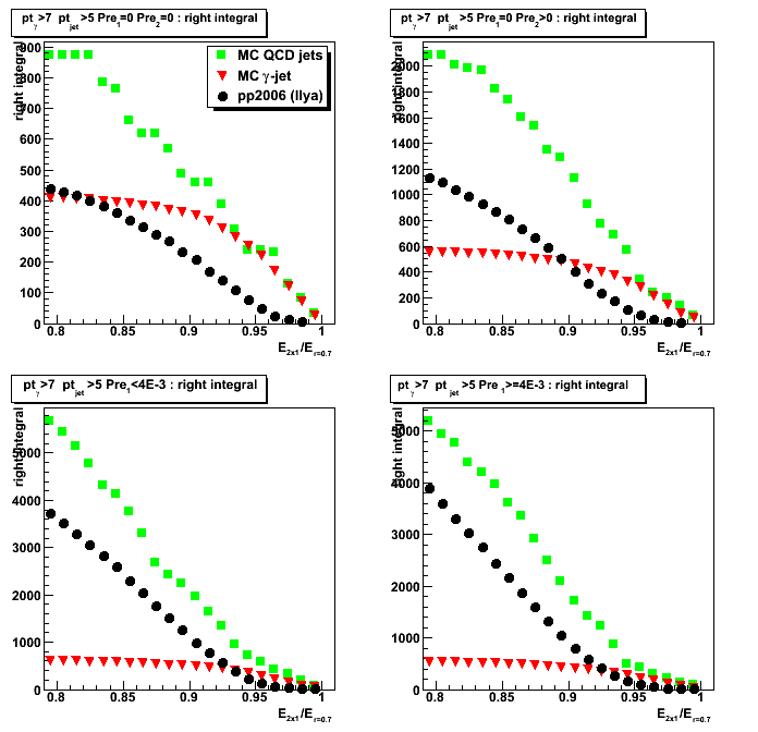
Figure 2c: 2x2/0.7 ratio

Figure 3c: 3x3/0.7 ratio

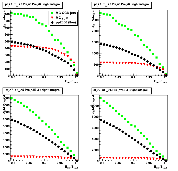
Figure 4c: 3x3/0.7 ratio but only using towers which passed jet finder threshold

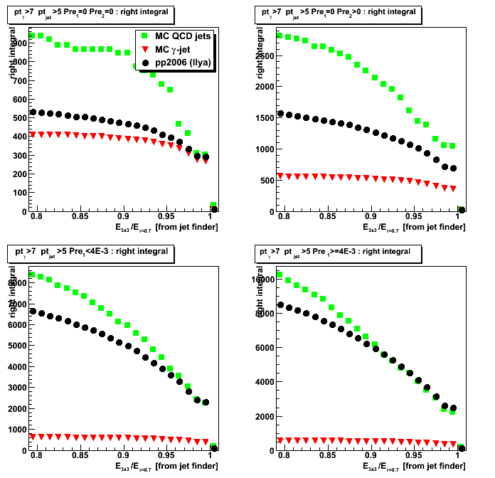
2008.11.21 Energy fraction from 2x1 vs. 2x2 vs. 3x3 or 0.7 radius: rapidity dependence

Ilya Selyuzhenkov November 21, 2008

Data sets:

pp2006 - STAR 2006 pp longitudinal data (~ 3.164 pb^1)
after applying gamma-jet isolation cuts (no R_cluster cut applied for this study).
gamma-jet[gamma-filtered] - data-driven Prompt Photon [p6410EemcGammaFilter] events.
Partonic pt range 2-25 GeV.
QCD jets[gamma-filtered] - data-driven QCD [p6410EemcGammaFilter] events.
Partonic pt range 2-25 GeV.

2x1, 2x2, and 3x3 clusters definition:

3x3 cluster: tower energy sum for 3x3 patch around highest tower
2x2 cluster: tower energy sum for 2x2 patch
which are closest to 3x3 tower patch centroid.
3x3 tower patch centroid is defined based
on tower energies weighted wrt tower centers:
centroid = sum{E_tow * r_tow} / sum{E_tow}.
Here r_tow=(x_tow, y_tow) denotes tower center.
2x1 cluster: tower energy sum for high tower plus second highest tower in 3x3 patch
r=0.7 energy is calculated based on towers
within a radius of 0.7 (in delta phi and eta) from high tower

Cuts applied

all gamma-jet candidate selection cuts except 3x3/r=0.7 energy isolation cut

Results

There are two sets of figures in links below:

Number of counts for a given energy fraction
Yield above given energy fraction
[figures with right integral in the caption]

Yield is defined as the integral above given energy fraction
up to the maximum value of 1

Gamma candidate detector eta < 1.5
(eta region where we do have most of the TPC tracking):

Gamma candidate detector eta > 1.5:
(smaller tower size)

Some observation

For pre1>0 condition (contains most of events)
yield in Monte-Carlo for eta > 1.5 case
is about factor of two different than that from pp2006 data,
while for eta < 1.5 Monte-Carlo yield agrees with data within 10-15%.
This could be due to trigger effect?
For pre1=0 case yiled for both eta > 1.5 and eta < 1.5 are different in data and MC
This could be due to migration of counts from pre1=0 to pre1>0
in pp2006 data due to more material budget than it is Monte-Carlo
For pre1=0 condition pp2006 data shapes are not reproduced by gamma-jet Monte-Carlo.
With a larger cluster size (2x1 -> 3x3) the pp2006 and MC gamma-jet shapes
are getting closer to each other.
For pre1>0 condition (with statistics available),
pp2006 data shapes are consistent with QCD Monte-Carlo.

Cluster energy fraction in 3x3 patch: detector eta > 1.5

Energy fraction from NxN cluster in 3x3 patch: detector eta > 1.5

Figure 1a: 2x1/3x3 energy fraction [number of counts per given fraction]

Figure 2a: 2x2/3x3 energy fraction [number of counts per given fraction]

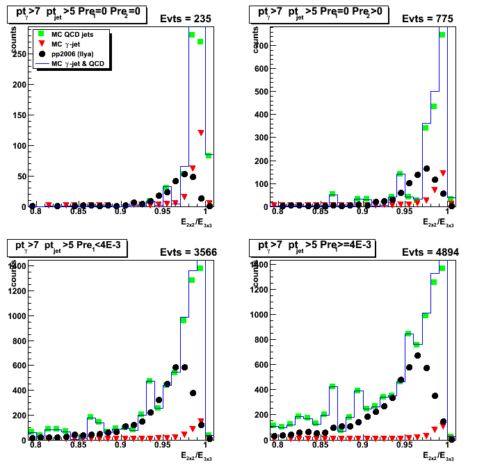
Yield vs. NxN cluster energy fraction in 3x3 patch: detector eta > 1.5

Figure 4a: 2x1/3x3 energy fraction [yield]

Figure 5a: 2x2/3x3 energy fraction [yield]

2008.11.25 Yiled vs. analysis cuts: eta dependence

Ilya Selyuzhenkov November 25, 2008

Data sets:

pp2006 - STAR 2006 pp longitudinal data (~ 3.164 pb^1)
gamma-jet[gamma-filtered] - data-driven Prompt Photon [p6410EemcGammaFilter] events.
Partonic pt range 2-25 GeV.
QCD jets[gamma-filtered] - data-driven QCD [p6410EemcGammaFilter] events.
Partonic pt range 2-25 GeV.

Some observation

Fig. 1 [upper&lower left, 3rd bin] indicates that
cluster energy isolation is the most important cut
for signal/background separation
Fig.1 [lower right, 3rd bin] shows that
R_cluster cut is independent from (or orthogonal to) other cuts
Fig.1 [upper&lower left 4th bin] shows that
cut on neutral energy fraction for the away side jet
rejects more signal that background events
We probably need to reconsider that cut
Fig.2 [lower left, 5th bin] shows that
charge particle veto significantly improves
signal to background ratio

Fig.2 [lower right, 5th bin] shows that
charge particle veto also independent from other cuts

Fig.3 [lower left, 5th bin] shows that
in the region were we do not have TPC tracking (photon eta > 1.5)
charge particle veto is not efficient,
although there is still some improvement from this cut.
This probably due to tracks with eta <1.5
which fall into large isolation radius r=0.7.

Yield vs. various analysis cuts

List of cuts (sorted according to bin number in Figs. 1-3. [No SMD sided residual cuts]):

N_events : total number of di-jet events found by the jet-finder
cos(phi_gamma - phi_jet) < -0.8 : gamma-jet opposite in phi
R_{3x3cluster}: Energy in 3x3 cluster of EEMC tower to the total jet energy
R_{3x3cluster}>0.9 for Fig. 1, and it is disabled in Fig. 2 and 3
R_EM^jet < 0.9 : neutral energy fraction cut for on away side jet
N_ch=0 : no charge tracks associated with a gamma candidate
N_bTow = 0 : no barrel towers associated with a gamma candidate (gamma in the endcap)
N_(5-strip cluster)^u > 2 : minimum number of strips in EEMC SMD u-plane cluster around peak
N_(5-strip cluster)^v > 2 : minimum number of strips in EEMC SMD v-plane cluster around peak
gamma-algo fail : my algorithm failed to match tower with SMD uv-intersection, etc...
Tow:SMD match : SMD uv-intersection has a tower which is not in a 3x3 cluster

Figure 1: Number of accepted events vs. various analysis cuts
The starting number of events (shown in first bin of the plots) is
the number of di-jets with reconstructed gamma_pt>7 GeV and jet_pt>5 GeV
upper left: cuts applied independently
upper right: expept this cut fired
(event passed all other cuts and being rejected by this cut)
lower left: "cuts applied independently" normalized by the total number of events
lower right: "expept this cut fired" normalized by the total number of events

Figure 2: Same as Fig.1 except: no R_cluster cut and photon detector eta < 1.5
(eta region where we do have most of the TPC tracking)

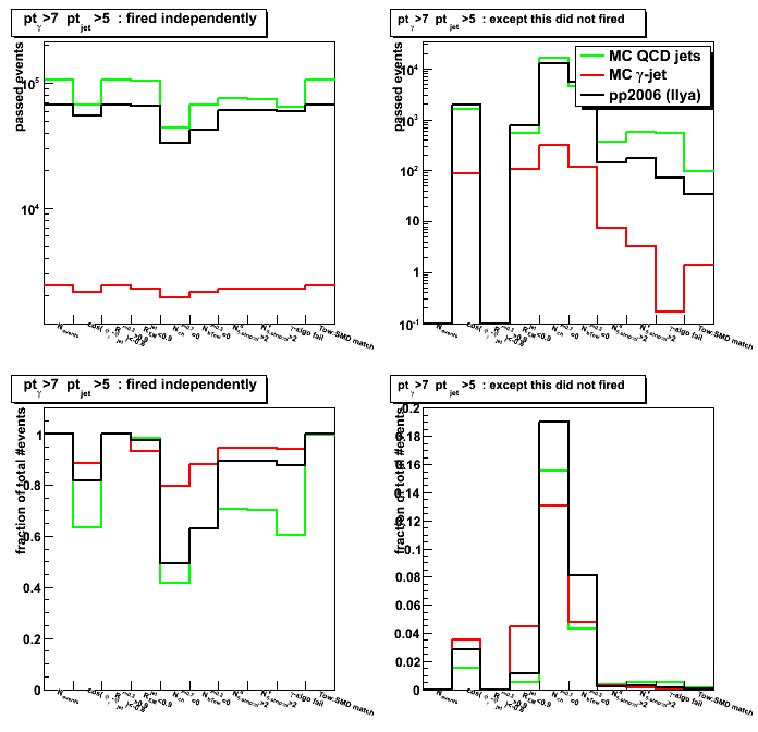
Figure 3: Same as Fig.1 except: no R_cluster cut and photon detector eta > 1.5

12 Dec

December 2008 posts

2008.12.08 Run 8 EEMC QA

Ilya Selyuzhenkov December 08, 2008

Data sets:

pp2006 - STAR 2006 pp longitudinal data (~ 3.164 pb^1)
Trigger: eemc-http-mb-L2gamma [id:137641]
pp2008 - STAR 2008 pp data
Trigger: etot-mb-l2 [id:7]
Days: 53-70; ~0.5M triggered events (1/3 of available statistics)

Detector subsystems involved in analysis:

TPC (vertex, jets, charge particle veto)
Endcap EMC (triggering, photon candidate reconstruction)
Barrel EMC (away side jet reconstruction)

Gamma-jet analysis cuts:

Select only di-jet events
cos(phi_gamma - phi_jet) < -0.8 : gamma-jet opposite in phi
R_EM^jet < 0.9 : neutral energy fraction cut for the away side jet
N_ch=0 : no charge tracks associated with a gamma candidate
N_bTow = 0 : no barrel towers associated with a gamma candidate (gamma in the endcap)
N_(5-strip cluster)^u > 2 : minimum number of strips in EEMC SMD u-plane cluster around peak
N_(5-strip cluster)^v > 2 : minimum number of strips in EEMC SMD v-plane cluster around peak
gamma-algo fail : my algorithm failed to match tower with SMD uv-intersection, etc...
Tow:SMD match : SMD uv-intersection has a tower which is not in a 3x3 cluster
R_{3x3cluster}: Energy in 3x3 cluster of EEMC tower to the total jet energy (not applied here)

Figure 1: EEMC x vs. y position of photon candidate for 2008 data sample
Problem with pre-shower layer in Sector 10 can been seen in the upper left corner

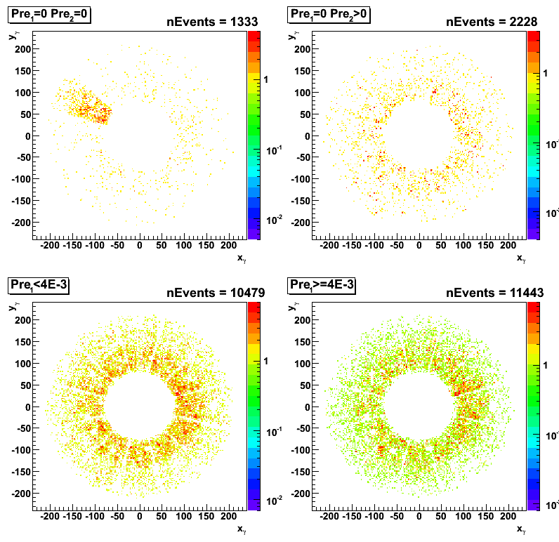
Figure 2: EEMC x vs. y position of photon candidate for 2006 data sample

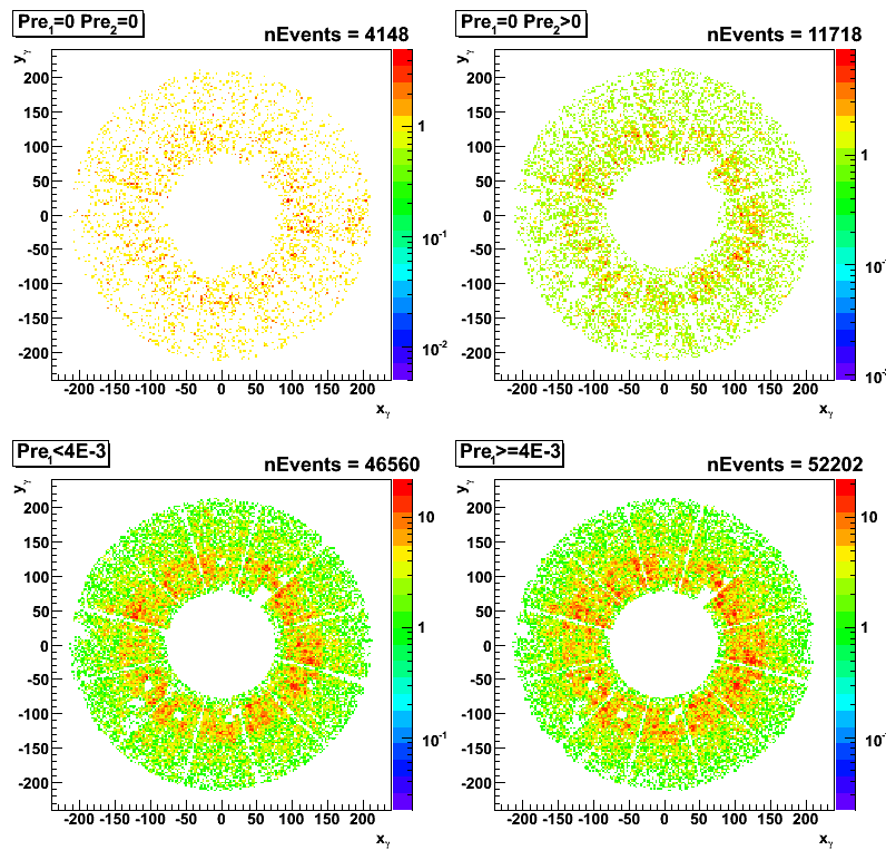
Figure 3: Average < E_pre1 * E_pre2 > for 3x3 cluster around high tower
vs run number for sectors 9, 10 and 11
Note, zero pre-shower energy for sector 10 (black points) for days 61, 62, 64, and 67.
All di-jet events for pp2008 data are shown (no gamma-jet cuts)

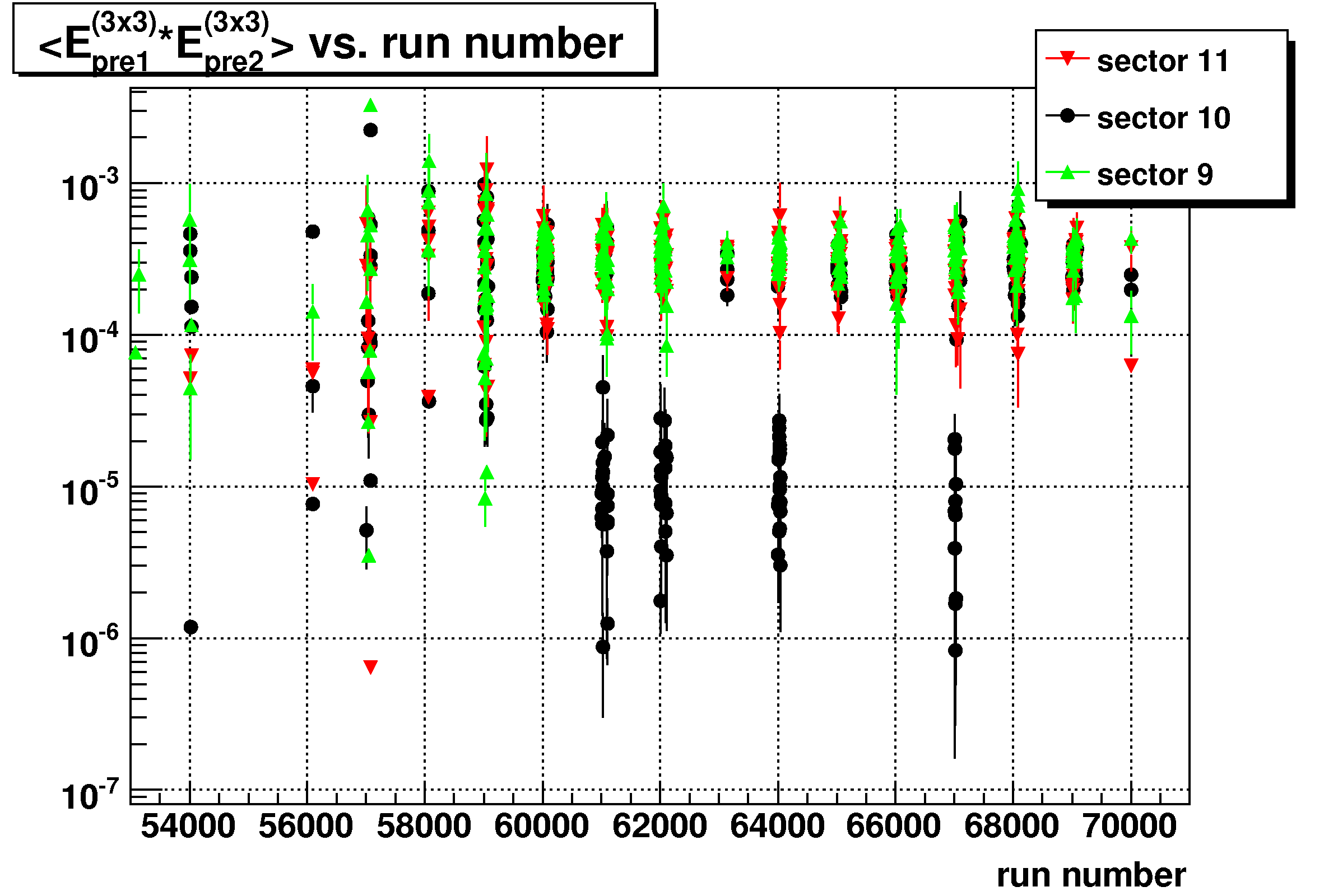
Figure 3a: Same as Fig.3, zoom into day 61

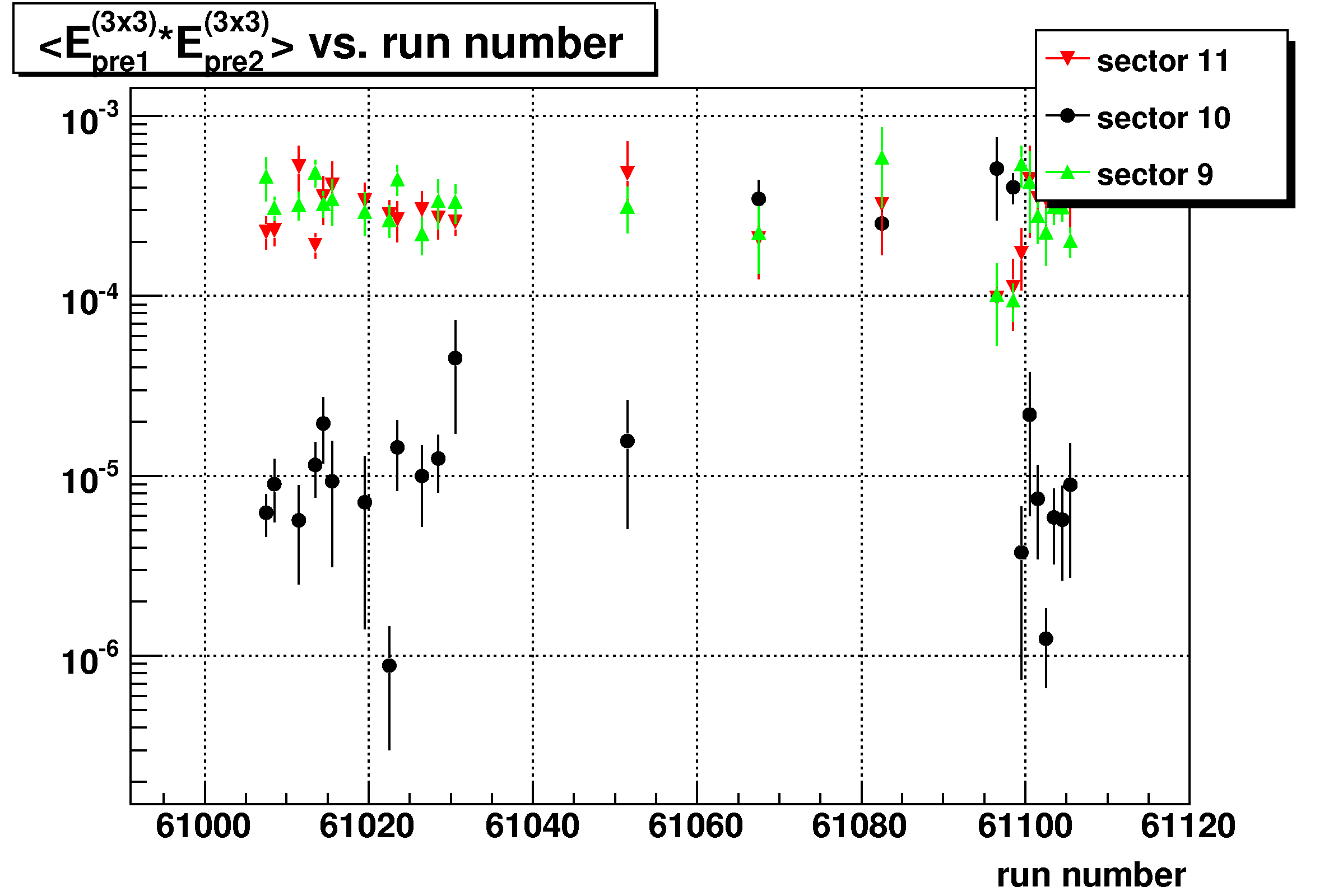
Figure 3b: Same as Fig.3, zoom into day 62
Figure 3c: Same as Fig.3, zoom into day 64
Figure 3d: Same as Fig.3, zoom into day 67

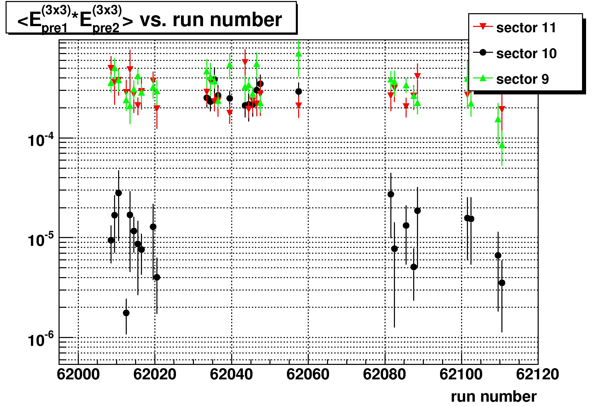
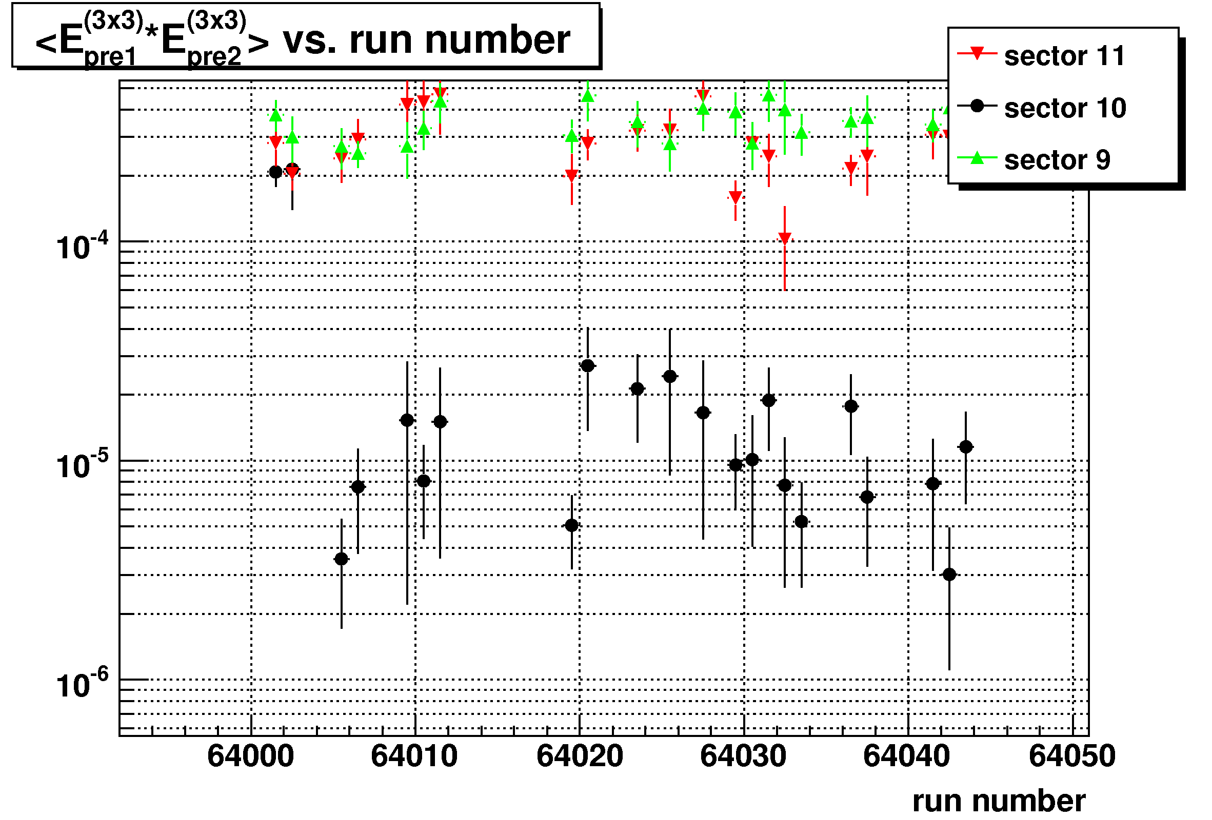
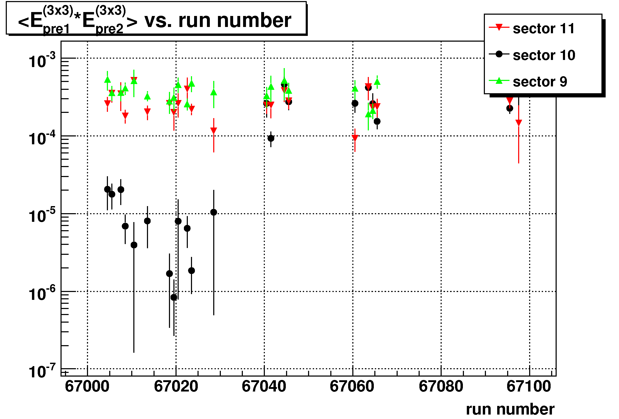
Figure 4: EEMC x vs. y position of photon candidate for 2008 data sample
Same as Fig. 1, but excluding days: 61, 62, 64, and 67

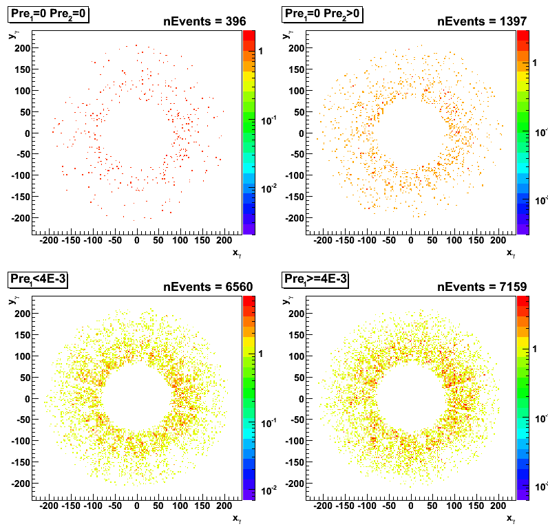
Conclusion on QA:

No problem with pp2008 data have been found,
except that for some runs (mostly on days 61, 62, 64, and 67)
EEMC pre-shower layer for sector 10 was off.

Comparison between 2006 and 2008 data

Figure 5: Vertex z distribution:
All gamma-jet cuts applied, plus pt_gamma>7 and pt_jet > 5 GeV (exlcuding days 61, 62, 64, and 67)
Results are shown for pp2008 data sample (black), vs. pp2006 data (red).
pp2008 data scaled to the same total number of candidates as in pp2006 data.

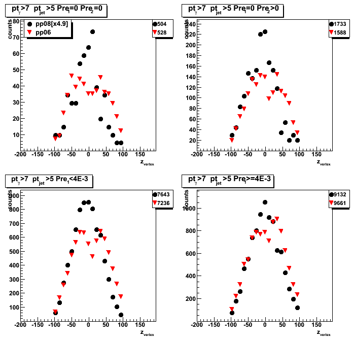
Figure 6: Shower shapes within +/- 30 strips from high strip (same cuts as in Fig. 5):

Figure 7: Shower shapes within +/- 5 strips from high strip
(same cuts as in Fig. 5, no scaling):

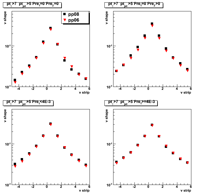
2008.12.09 pp Run 8 vs. Run 6 SMD shower shapes

Ilya Selyuzhenkov December 09, 2008

Data sets:

pp2006 - STAR 2006 pp longitudinal data (~ 3.164 pb^1)
Trigger: eemc-http-mb-L2gamma [id:137641]
pp2008 - STAR 2008 pp data
Trigger: etot-mb-l2 [id:7]
Days: 53-70; ~0.5M triggered events (1/3 of available statistics)

2008.12.09 pp Run 8 vs. Run 6 SMD shower shapes

Ilya Selyuzhenkov December 09, 2008

Data sets:

pp2006 - STAR 2006 pp longitudinal data (~ 3.164 pb^1)
Trigger: eemc-http-mb-L2gamma [id:137641]
pp2008 - STAR 2008 pp data
Trigger: etot-mb-l2 [id:7]
Days: 53-70; ~0.5M triggered events (1/3 of available statistics)

Gamma-jet analysis cuts:

Select only di-jet events
cos(phi_gamma - phi_jet) < -0.8 : gamma-jet opposite in phi
R_EM^jet < 0.9 : neutral energy fraction cut for the away side jet
N_ch=0 : no charge tracks associated with a gamma candidate
N_bTow = 0 : no barrel towers associated with a gamma candidate (gamma in the endcap)
N_(5-strip cluster)^u > 2 : minimum number of strips in EEMC SMD u-plane cluster around peak
N_(5-strip cluster)^v > 2 : minimum number of strips in EEMC SMD v-plane cluster around peak
gamma-algo fail : my algorithm failed to match tower with SMD uv-intersection, etc...
Tow:SMD match : SMD uv-intersection has a tower which is not in a 3x3 cluster
R_{3x3cluster}: Energy in 3x3 cluster of EEMC tower to the total jet energy (not applied here)

Comparison between 2006 and 2008 data

Figure 1: Vertex z distribution:
All gamma-jet cuts applied, plus pt_gamma>7 and pt_jet > 5 GeV (exlcuding days 61, 62, 64, and 67)
Results are shown for pp2008 data sample (black), vs. pp2006 data (red).
pp2008 data scaled to the same total number of candidates as in pp2006 data.

Figure 2: Shower shapes within +/- 30 strips from high strip (same cuts as in Fig. 1):

Figure 3: Shower shapes within +/- 5 strips from high strip
(same cuts as in Fig. 1, no scaling):

2008.12.09 pp Run 8 vs. Run 6 SMD shower shapes

Ilya Selyuzhenkov December 09, 2008

Data sets:

pp2006 - STAR 2006 pp longitudinal data (~ 3.164 pb^1)
Trigger: eemc-http-mb-L2gamma [id:137641]
pp2008 - STAR 2008 pp data
Trigger: etot-mb-l2 [id:7]
Days: 53-70; ~0.5M triggered events (1/3 of available statistics)

Gamma-jet analysis cuts:

Select only di-jet events
cos(phi_gamma - phi_jet) < -0.8 : gamma-jet opposite in phi
R_EM^jet < 0.9 : neutral energy fraction cut for the away side jet
N_ch=0 : no charge tracks associated with a gamma candidate
N_bTow = 0 : no barrel towers associated with a gamma candidate (gamma in the endcap)
N_(5-strip cluster)^u > 2 : minimum number of strips in EEMC SMD u-plane cluster around peak
N_(5-strip cluster)^v > 2 : minimum number of strips in EEMC SMD v-plane cluster around peak
gamma-algo fail : my algorithm failed to match tower with SMD uv-intersection, etc...
Tow:SMD match : SMD uv-intersection has a tower which is not in a 3x3 cluster
R_{3x3cluster}: Energy in 3x3 cluster of EEMC tower to the total jet energy (not applied here)

Comparison between 2006 and 2008 data

Figure 2: Shower shapes within +/- 30 strips from high strip (same cuts as in Fig. 1):

Figure 3: Shower shapes within +/- 5 strips from high strip
(same cuts as in Fig. 1, no scaling):

2008.12.09 pp Run 8 vs. Run 6 SMD shower shapes

Ilya Selyuzhenkov December 09, 2008

Data sets:

pp2006 - STAR 2006 pp longitudinal data (~ 3.164 pb^1)
Trigger: eemc-http-mb-L2gamma [id:137641]
pp2008 - STAR 2008 pp data
Trigger: etot-mb-l2 [id:7]
Days: 53-70; ~0.5M triggered events (1/3 of available statistics)

Gamma-jet analysis cuts:

Select only di-jet events
cos(phi_gamma - phi_jet) < -0.8 : gamma-jet opposite in phi
R_EM^jet < 0.9 : neutral energy fraction cut for the away side jet
N_ch=0 : no charge tracks associated with a gamma candidate
N_bTow = 0 : no barrel towers associated with a gamma candidate (gamma in the endcap)
N_(5-strip cluster)^u > 2 : minimum number of strips in EEMC SMD u-plane cluster around peak
N_(5-strip cluster)^v > 2 : minimum number of strips in EEMC SMD v-plane cluster around peak
gamma-algo fail : my algorithm failed to match tower with SMD uv-intersection, etc...
Tow:SMD match : SMD uv-intersection has a tower which is not in a 3x3 cluster
R_{3x3cluster}: Energy in 3x3 cluster of EEMC tower to the total jet energy (not applied here)

Comparison between 2006 and 2008 data

Figure 2: Shower shapes within +/- 30 strips from high strip (same cuts as in Fig. 1):

Figure 3: Shower shapes within +/- 5 strips from high strip
(same cuts as in Fig. 1, no scaling):

2008.12.09 pp Run 8 vs. Run 6 SMD shower shapes

Ilya Selyuzhenkov December 09, 2008

Data sets:

pp2006 - STAR 2006 pp longitudinal data (~ 3.164 pb^1)
Trigger: eemc-http-mb-L2gamma [id:137641]
pp2008 - STAR 2008 pp data
Trigger: etot-mb-l2 [id:7]
Days: 53-70; ~0.5M triggered events (1/3 of available statistics)

Gamma-jet analysis cuts:

Select only di-jet events
cos(phi_gamma - phi_jet) < -0.8 : gamma-jet opposite in phi
R_EM^jet < 0.9 : neutral energy fraction cut for the away side jet
N_ch=0 : no charge tracks associated with a gamma candidate
N_bTow = 0 : no barrel towers associated with a gamma candidate (gamma in the endcap)
N_(5-strip cluster)^u > 2 : minimum number of strips in EEMC SMD u-plane cluster around peak
N_(5-strip cluster)^v > 2 : minimum number of strips in EEMC SMD v-plane cluster around peak
gamma-algo fail : my algorithm failed to match tower with SMD uv-intersection, etc...
Tow:SMD match : SMD uv-intersection has a tower which is not in a 3x3 cluster
R_{3x3cluster}: Energy in 3x3 cluster of EEMC tower to the total jet energy (not applied here)

Comparison between 2006 and 2008 data

Figure 2: Shower shapes within +/- 30 strips from high strip (same cuts as in Fig. 1):

Figure 3: Shower shapes within +/- 5 strips from high strip
(same cuts as in Fig. 1, no scaling):

Conclusion:

2008.12.09 pp Run 8 vs. Run 6 shower shapes

Ilya Selyuzhenkov December 09, 2008

Data sets:

pp2006 - STAR 2006 pp longitudinal data (~ 3.164 pb^1)
Trigger: eemc-http-mb-L2gamma [id:137641]
pp2008 - STAR 2008 pp data
Trigger: etot-mb-l2 [id:7]
Days: 53-70; ~0.5M triggered events (1/3 of available statistics)

Gamma-jet analysis cuts:

Select only di-jet events
cos(phi_gamma - phi_jet) < -0.8 : gamma-jet opposite in phi
R_EM^jet < 0.9 : neutral energy fraction cut for the away side jet
N_ch=0 : no charge tracks associated with a gamma candidate
N_bTow = 0 : no barrel towers associated with a gamma candidate (gamma in the endcap)
N_(5-strip cluster)^u > 2 : minimum number of strips in EEMC SMD u-plane cluster around peak
N_(5-strip cluster)^v > 2 : minimum number of strips in EEMC SMD v-plane cluster around peak
gamma-algo fail : my algorithm failed to match tower with SMD uv-intersection, etc...
Tow:SMD match : SMD uv-intersection has a tower which is not in a 3x3 cluster
R_{3x3cluster}: Energy in 3x3 cluster of EEMC tower to the total jet energy (not applied here)

Comparison between 2006 and 2008 data

Figure 2: Shower shapes within +/- 30 strips from high strip (same cuts as in Fig. 1):

Figure 3: Shower shapes within +/- 5 strips from high strip
(same cuts as in Fig. 1, no scaling):

2008.12.11 Run 8 EEMC QA (presentation for Spin PWG)

Ilya Selyuzhenkov December 11, 2008

Run 8 QA with EEMC gamma-jet candidates

Presentation in pdf or open office file format

2008.12.16 Effect of L2gamma trigger in simulations

Ilya Selyuzhenkov December 16, 2008

Data sets

pp2006 - STAR 2006 pp longitudinal data (~ 3.164 pb^1)
Trigger: eemc-http-mb-L2gamma [id:137641]
gamma-jet[gamma-filtered] - data-driven Prompt Photon [p6410EemcGammaFilter] events.
Partonic pt range 2-25 GeV.
QCD jets[gamma-filtered] - data-driven QCD [p6410EemcGammaFilter] events.
Partonic pt range 2-25 GeV.

Cuts applied

Gamma-jet isolation cuts except 3x3/r=0.7 energy isolation cut

Data driven shower shape replacement maker fix

Figure 1: (reproducing old results with dd-maker fix)
transverse momentum and vertex z distributions
before (with ideal gains/pedestals) and
after (with realistic gains/pedestal tables) dd-maker fix are in a good agreement.
For details on "dd-maker problem", read these hyper news threads:
emc2:2905, emc2:2900, and phana:294
Now we can run L2gamma trigger emulation and Eemc SMD ddMaker
in the same analysis chain.

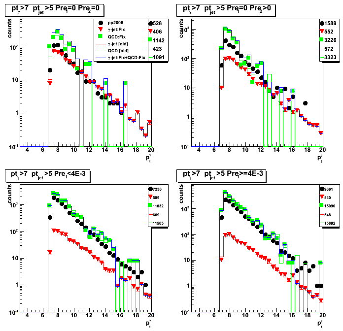
l2-gamma trigger effect in simulation

Figure 2: Vertex z distribution with and without trigger condition in simulations
(emulated trigger: eemc-http-mb-L2gamma [id:137641]).
Solid red/green symbols show results with l2gamma condition applied,
while red/green lines show results for the same analysis cuts but without trigger condition.
Note, good agreement between MC QCD jets with trigger condition on (green solid squared)
and pp2006 data (black solid circles) for pre-shower1>0 case.

Figure 3: pt distribution with/without trigger condition in simulations.
Same color coding as in Fig. 2

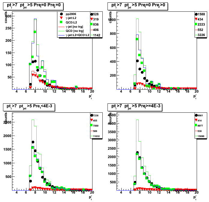
Figure 4: Same as Fig. 3 just on a log scale
One can clearly see large trigger effect when applied for QCD jet events,
and a little effect for direct gammas.

Figure 5: gamma candidate pt QCD (right) and prompt photon (left) Monte-Carlo:
no (upper) with (lower) L2e-gamma trigger condition
No photon pt and no jet pt cuts

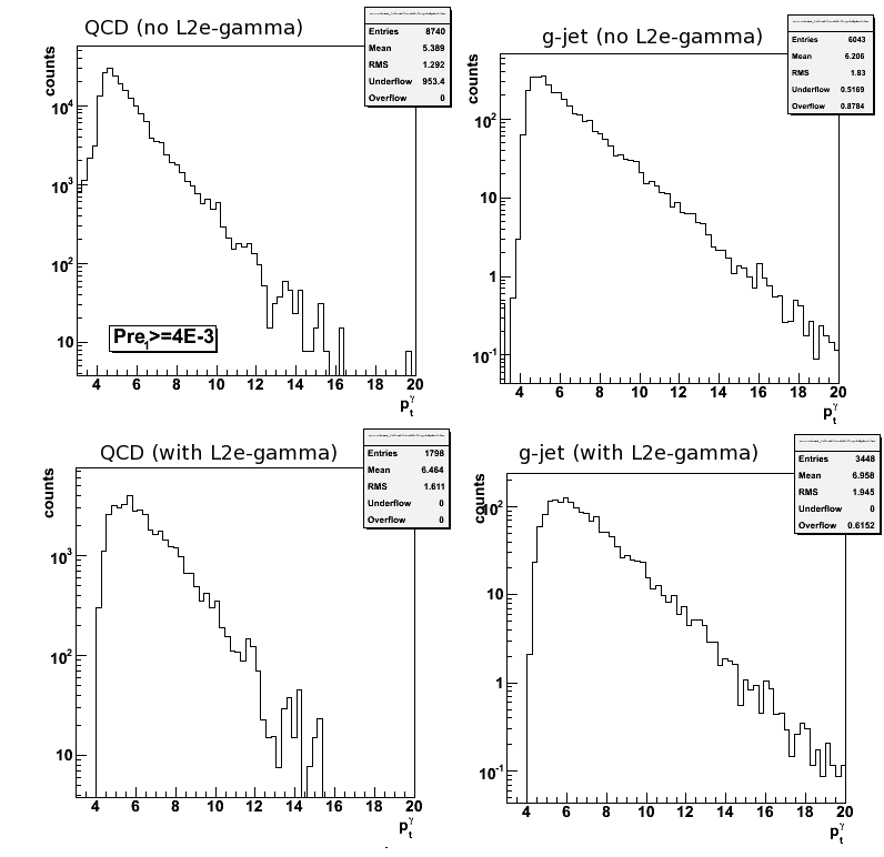
Figure 6: gamma candidate pt for QCD Monte-Carlo: no L2e-gamma trigger condition
No photon pt and no jet pt cuts

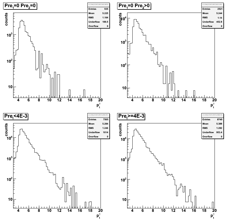
Figure 7: gamma candidate pt for QCD Monte-Carlo: L2e-gamma trigger condition applied (id:137641)
No photon pt and no jet pt cuts

2008.12.19 Parton pt distribution for Pythia QCD and gamma-jet events

Ilya Selyuzhenkov December 19, 2008

Data sets

gamma-jet[gamma-filtered] - data-driven Prompt Photon [p6410EemcGammaFilter] events.
Partonic pt range 2-25 GeV.
QCD jets[gamma-filtered] - data-driven QCD [p6410EemcGammaFilter] events.
Partonic pt range 2-25 GeV.

Cuts applied

Gamma-jet isolation cuts except 3x3/r=0.7 energy isolation cut

Figure 1: Parton pt distibution for gamma-jet candidates from Pythia QCD sample
with various pt and l2gamma trigger conditions

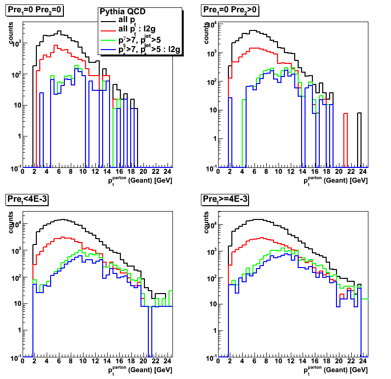
Figure 2: Parton pt distibution for gamma-jet candidates from Pythia prompt photon sample
with various pt and l2gamma trigger conditions