BSMD
Collected here is information about BSMD Calibrations.
There are 36,000 BSMD channels, divided into 18,000 strips in eta and 18,000 strips in phi. They are located 5.6 radiation lengths deep in the Barrel Electromagnetic Calorimeter (BEMC).
1) DATA: 2008 BSMD Calibration
Information about the 2008 BSMD Calibration effort will be posted below as sub-pages.
Fig 1. BSMD-E 2D mapping of soft ID. (plot for reverse mapping is attached)

01) raw spectra
Goals:
- verify pedestals loaded to DB are reasonable for 2008 pp data
- estimate stats needed to find slopes of individual strips for minB events
Method:
- look at pedestal residua for individual strips, exclude caps 1 & 2, use only status==1
- fit gauss & compare with histo mean
- find integrals of individual strips, sum over 20 ADC channels starting from ped+5*sig
To obtain muDst w/o zero suppression I run privately the following production chain:
chain="DbV20080703 B2008a ITTF IAna ppOpt VFPPV l3onl emcDY2 fpd ftpc
trgd ZDCvtx NosvtIT NossdIT analysis Corr4 OSpaceZ2 OGridLeak3D
beamLine BEmcDebug"
Fig 1
Examples of single strip pedestal residua, based on ~80K minB events from days 47-65, 30 runs. (1223 is # of bins, ignore it).
Left is typical good spectrum, see Fig2.3. Middle is also reasonable, but peds is 8 channels wide vs. typical 4 channels.
The strip shown on the right plot is probably broken.

Fig 2
Detailed view on first 500 strips. X=stripID for all plots.
- Y=mean of the gauss fit to pedestal residuum, in ADC channels, error=sigma of the gauss.
- Y=integral of over 20 ADC channels starting from ped+5*sig.
- Raw spectra, Y=ADC-ped, exclude caps 1 & 2, use only status==1

Fig 3
Broader view of ... problems in BSMD-E plane. Note, status flag was taken in to account.
Top plot is sum of 30 runs from days 47-65, 80K events. Bottom plot is just 1 run, 3K events. You can't distinguish individual channels, but scatter plot works like a sum of channels, so it is clear the slopes are there, we need just more data.

Conclusions:
- DB peds for BSMDE look good on average.
- with 1M eve we will start to see gains for individual strip relativewith ~20% error. Production will finish tomorrow.
- there are portions of SMDE masked out (empty area in fig 3.2, id=1000) - do why know what broke? Will it be fixed in 2009 run
- there are portions of SMDE not masked but dead (solid line in fig 3.2, id=1400) - worth to go after those
- there are portions of SMDE not masked with unstable (or wrong) pedestal, (fig 3.1 id=15000)
- for most channels there is one or more caps with different ped not accounted for in DB ( thin line below pedestal in fig 2.3)
- One gets a taste of gain variation from fig 2.2
- Question: what width of pedestal is tolerable. Fig 2.1 shows width as error bars. Should I kill channel ID=152?
02) relative BSMD-E gains from 1M dAu events
Glimpse of relative calibration of BSMDE from 2008 d+Au data
Input: 1M dAu minb events from runs: 8335112+8336019
Method : fit slopes to individual strips, as discussed 01) raw spectra
Fig 1
Examples of raw pedestal corrected spectra for first 9 strips, 1M dAu events

Fig 2
Detailed view on first 500 strips. X=stripID for all plots.
- Y=mean of the gauss fit to pedestal residuum, in ADC channels, error=sigma of the gauss.
- Y=integral of over 20 ADC channels starting from ped+5*sig. Raw spectra,
- Y=gain defined as "-slope" from the exponential fit over ADC range 20-40 channels, errors from expo fit. Blue line is constant fit to gains.

Fig 3
BSMDE strips cover the whole barrel and eta-phi representation is better suited to present 18K strips in one plot.
- Mapping of BSMDE-softID (Z-axis) in to eta-phi space. Eta bin 0 is eta=-1.0, eta bin 299 is eta=+1.0. Phi bin 0 starts at 12:30 and advances as phi angle.
- gains for majority of 18K BSMDE strips. White means no data or discarded by rudimentary QA of peds, yields or slope.

Fig 4
For reference spectra from 1M pp events from ~12 EmcCheck runs from days 47-51. It proves I did it and it was naive on my side to expect 1M pp events is enough.

Fig 5
More pp events spectra - lot of problems with DB content.

03) more details , answering Will
This page provides more details addressing some of Will's questions.
2) fig 2: well, 500 chns is not a very "natural" unit, but I wonder
what corresponds to 50 chns (e.g., the region of fluctuation
250-300) ... I need to check my electronics readout diagrams
again, or maybe folks more expert will comment
Fig 1.
Zoom-in of the god-to-bad region of BSMDE

Fig 2.
'Good' strips belong to barrel module 2, crate 2, sitting at ~1 o'cloCk on the WEST

Fig 3.
'BAD' strips belong also to barrel module 2, crate 2, sitting at ~1 o'cloCk on the WEST

04) bad CAP 123
Study of pedestal correlation for BSMDE
Goal: identify source of the band below main pedestals.
Figs 1,2 show pedestals 'breathe' in correlated way for channels in the same crate, but this mode is decoupled between crates. It may be enough to use individual peds for all CAPS to reduce this correlation.
Fig3 shows CAP=123 has bi-modal pedestals. FYI, CAPS 124,125 were excluded because they also are different.
Based on Fig1 & 3 one could write an algo identifying event by event in which mode CAP=123 settled, but for now I'll discard CAP123 as well.
All plots are made based on 500K d-Au events from the run 8336052.
Fig 0
Example of pedestal residua for BSMDE strips 1-500, after CAPS 124 and 125 were excluded.

Fig 1
Correlation between pedestal residua for neighbor strips. Strip 100 is used on all plots on the X-axis

Fig 2
Correlation between pedestal residua for strips in different crates. Strip 100 is used on all plots on the X-axis

Fig 3
Squared pedestal residua for strips [1,150] were summed for every event and plotted as function of CAP ID (Y-axis).
Those strips belong to the same module #1 . X-axis shoes SQRT(sum) for convenience. CAP=123 has double pedestal.

05) BSMDE saturation, dAu, 500K minB eve
Input: 500K d-Au events from run 8336052,
Method : drop CAPS 123,124,125, subtract single ped for all other CAPS.
Fig 1 full resolution, only 6 modules , every module contains 150 strips.
Fig 2 All 18K strips (120 modules), every module contain only 6 bins, every bin is sum of 25 strips.
h->RebinX(25), h->SetMinimum(2), h->SetMaximum(1e5)

06) QAed relative gains BSMDE, 3M d-Au events , ver1.0
Version 1 of relative gains for BSMDE, d-AU 2008.
INPUT: 3M d-AU events from day ~336 of 2007.
Method: fit slopes to ADC =ped+30,ped+100.
The spectra, fits of pedestal residuum, and slopes were QAed.
Results: slopes were found for 16,577 of 18,000 strips of BSMDE.
Fig1 Good spectrum for strip ID=1. X-axis ADC-ped, CAPs=123,124,124 excluded.

Fig2 TOP: slopes distribution (Y-axis) vs. stripID within given module ( X-axis). Physical eta=0.0 is at X=0, eta=1.0 is at X=150.
BOTTOM: status tables with marked eta-phi location excluded 1423 strips of BSMDE by multi-stage QA of the spectra. Different colors denote various failed tests.

Fig3 Mapping of known BSMDE topology on chosen by us eta-phi 2D localization. Official stripID is shown in color.
07) QA method for SMD-E, slopes , ver1.1
Automatic QA of BSMDE minB spectra.
Content
- example of good spectra (fig 0)
- QA cuts definition (table 1) + spectra (figs 1-7)
- Result:
- # of bad strips per module. BSMDE modules 10,31,68 are damaged above 50%+. (modules 16-30 served by crate 4 were not QAed).
- eta-phi distributions of: slopes, slope error (fig 9) , pedestal, pedestal (fig 10) width _after_ QA
- sample of good and bad plots from every module, including modules 16-30 (PDF at the end)
The automatic procedure doing QA of spectra was set up in order to preserve only good looking spectra as shown in the fig 0 below.
Fig 0 Good spectra for random strips in module=2. X-axis shows pedestal residua. It is shown to set a scale for the bad strips shown below.

INPUT: 3M d-AU events from day ~336 of 2007.
All spectra were pedestals subtracted, using one value per strip, CAPS=123,124,125 were excluded. Below I'll use term 'ped' instead of more accurate pedestal residuum.
Method: fit slopes to ADC =ped+40,ped+90 or 5*sig(ped) if too low.
The spectra, fits of pedestal residuum, and slopes were QAed.
QA method was set up as sequential series of cuts, upon failure later cuts were not checked.
Note, BSMD rate 4 had old resistors in day 366 of 2007 and was excluded from this analysis.
This reduces # of strips from 18,000 to 15,750 .
| cut# | cut code | description | # of discarded strips | figure |
| 1 | 1 | at least 10,000 entries in the MPV bin | 4 | - |
| 2 | 2 | MPV position within +/-5 ADC channels | 57 | Fig 1 |
| 3 | 4 | sig(ped) of gauss fit in [1.6,8] ADC ch | 335 | Fig 2 |
| 4 | 8 | position of mean gauss within +/- 4 ADC | 11 | Fig 3 |
| 5 | 16 | yield from [ped+40,ped+90] out of range | 441 | Fig 4 |
| 6 | 32 | chi2/dof from slop fit in [0.6,2.5] | 62 | Fig 5 |
| 7 | 64 | slopeError/slop >16% | 4 | Fig 6 |
| 8 | 128 | slop within [-0.015, -0.05] | 23 | Fig 7 |
| - | sum | out of processed 15,750 strips discarded | 937 ==> 5.9% |
Fig 1 Example of strips failing QA cut #2, MPV position out of range , random strip selection

Fig 2a Distribution of width of pedestal vs. eta-bin

Fig 2b Example of strips failing QA cut #3, width of pedestal out of range , random strip selection

Fig 3a Distribution of pedestal position vs. eta-bin

Fig 3b Example of strips failing QA cut #4, pedestal position out of range , random strip selection

Fig 4a Distribution of yield from the slope fit range vs. eta-bin

Fig 4b Example of strips failing QA cut #5, yield from the slope fit range out of range , random strip selection

Fig 5a Distribution of chi2/DOF from the slope fit vs. eta-bin

Fig 5b Example of strips failing QA cut #6, chi2/DOF from the slope fit out of range , random strip selection

Fig 6a Distribution of err/slope vs. eta-bin

Fig 6b Example of strips failing QA cut #7, err/slope out of range , random strip selection

Fig 7a Distribution of slope vs. eta-bin

Fig 7b Example of strips failing QA cut #8, slope out of range , random strip selection

Results
Fig 8a Distribution of # of bad strips per module.
BSMDE modules 10,31,68 are damaged above 50%+. Ymax was set to 150, i.e. to the # of eat strips per module. Modules 16-30 served by crate 4 were not QAed.

Fig 8b 2D Distribution of # of bad strips indexed by eta & phi strip location. Z-scale denotes error code from the 2nd column from table 1.

Fig 9 2D Distribution of slope indexed by eta & phi strip location.
TOP: slopes. There is room for gain improvement in the offline analysis. At fixed eta (vertical line) there should be no color variation.
BOTTOM error of slope/slope.

Fig 10 2D Distribution of pedestal and pedestal width indexed by eta & phi strip location.
TOP: pedestal
BOTTOM: pedestal width.

08) SMD-E gain equalization , ver 1.1
Goal : predict BSMD-E relative gain corrections for every eta bin
Method : find average slope per eta slice, fit gauss, determine average slope : avrSlope(iEta)
Gain correction formula is used only for extreme deviations:
- gainCorr_i = slope_i/avrSlope(iEta), i =1,..,18,000
- if( fabs(1-gainCorr)<0.15) gainCor=1.0 // do not correct
Fig 1 Example of 2 eta slices
 |  |
Fig 2 TOP: Slope distribution vs. eta-bin, average marked by crosses
BOTTOM: predicted gain correction. Correction=1 for strips w/ undetermined gains.

Fig 3 Predicted gain correction. Correction=1 for ~14K of 18K strips.

Fig 4 The same predicted gain correction vs. stripID.

09) QA of SMD-P slopes, ver1.1
Automatic QA of BSMD-P minB spectra.
Content
- example of good spectra (fig 0)
- QA cuts definition (table 1) + spectra (figs 1-7)
- Result:
- # of bad strips per module. BSMD-P modules 1,4,59,75,85 are damaged above 50%+. (modules 16-30 served by crate 4 were not QAed).
- eta-phi distributions of: slopes, slope error (fig 9) , pedestal, pedestal (fig 10) width _after_ QA
- sample of good and bad plots from every module, including modules 16-30 (PDF at the end)
The automatic procedure doing QA of spectra was set up in order to preserve only good looking spectra as shown in the fig 0 below.
Fig 0 Good spectra for random strips in module=2. X-axis shows pedestal residua. It is shown to set a scale for the bad strips shown below.

INPUT: 3M d-AU events from day ~336 of 2007.
All spectra were pedestals subtracted, using one value per strip, CAPS=123,124,125 were excluded. Below I'll use term 'ped' instead of more accurate pedestal residuum.
Method: fit slopes to ADC =ped+40,ped+90 or 5*sig(ped) if too low.
The spectra, fits of pedestal residuum, and slopes were QAed.
QA method was set up as sequential series of cuts, upon failure later cuts were not checked.
Note, BSMD rate 4 had old resistors in day 366 of 2007 and was excluded from this analysis.
This reduces # of strips from 18,000 to 15,750 .
| cut# | cut code | description | # of discarded strips | figure |
| 1 | 1 | at least 10,000 entries in the MPV bin | 2 | - |
| 2 | 2 | MPV position within +/-5 ADC channels | 10 | Fig 1 |
| 3 | 4 | sig(ped) of gauss fit in [0.75,8] ADC ch | 32 | Fig 2 |
| 4 | 8 | position of mean gauss within +/- 4 ADC | 0 | Fig 3 |
| 5 | 16 | yield from [ped+40,ped+90] out of range | 758 | Fig 4 |
| 6 | 32 | chi2/dof from slop fit in [0.55,2.5] | 23 | Fig 5 |
| 7 | 64 | slopeError/slop >10% | 1 | Fig 6 |
| 8 | 128 | slop within [-0.025, -0.055] | 6 | Fig 7 |
| - | sum | out of processed 15,750 strips discarded | 831 ==> 5.2% |
Fig 1 Example of strips failing QA cut #2, MPV position out of range , random strip selection

Fig 2a Distribution of width of pedestal vs. strip # inside the module. For the East side I cout strips as -1,-2, ...,-150.

Fig 2b Example of strips failing QA cut #3, width of pedestal out of range , random strip selection

Fig 3 Distribution of pedestal position vs. strip # inside the module

Fig 4a Distribution of yield from the slope fit range vs. eta-bin

Fig 4b Example of strips failing QA cut #5, yield from the slope fit range out of range , random strip selection

Fig 5a Distribution of chi2/DOF from the slope fit vs. eta-bin

Fig 5b Example of strips failing QA cut #6, chi2/DOF from the slope fit out of range , random strip selection

Fig 6 Distribution of err/slope vs. eta-bin

Fig 7a Distribution of slope vs. eta-bin

Fig 7b Example of strips failing QA cut #8, slope out of range , random strip selection

Results
Fig 8a Distribution of # of bad strips per module.
BSMD-P modules 1,4,59,75,85 are damaged above 50%+. Ymax was set to 150, i.e. to the # of eat strips per module. Modules 16-30 served by crate 4 were not QAed.

Fig 8b 2D Distribution of # of bad strips indexed by eta & phi strip location. Z-scale denotes error code from the 2nd column from table 1.

Fig 9 2D Distribution of slope indexed by eta & phi strip location.
TOP: slopes. At fixed eta (horizontal line) there should be no color variation. red=dead strips
BOTTOM error of slope/slope. white=dead strip

Fig 10 2D Distribution of pedestal and pedestal width indexed by eta & phi strip location.
TOP: pedestal. dead strip have 0 residuum.
BOTTOM: pedestal width. white marks dead strips

10) SMD-P gain equalization , ver 1.1
Goal : predict BSMD-P relative gain corrections for every eta bin
Method : find average slope per eta slice, fit gauss, determine average slope : avrSlope(iEta)
Gain correction formula is used only for extreme deviations:
- gainCorr_i = slope_i/avrSlope(iEta), i =1,..,18,000
- if( fabs(1-gainCorr)<0.10) gainCor=1.0 // do not correct
Fig 1 Example of 2 eta slices
 |  |
Fig 2 LEFT: Slope distribution vs. eta-bin, average marked by crosses
RIGHT: predicted gain correction. Correction=1 for strips w/ undetermined gains.

Fig 3 Predicted gain correction. Correction=1 for ~14K of 18K strips.

Fig 4 The same predicted gain correction vs. stripID.

12) investigating status of P-strips
Fig 1. West BSMD-P

Fig 2. East BSMD-P
p>
13) ver 1.2 : SMD-E, -P, status & relative gains, no Crate4
Automatic BSMD-E, -P relative calibration and status tables.
The second pass through both SMDE, SMDP was performed, learning from previous mistakes.
Main changes:
- relax most of the QA cuts
- smooth raw spectra to reduce significance 1-2 channels wide of spikes and deeps in raw spectra
- extend slop fit range to ped +[30,100]
- still do not use crate 4 - it has to many problems
- reduce margin for gain correction - now 10%+ deviation is corrected.
INPUT: 3M d-AU events from day ~336 of 2007.
All spectra were pedestals subtracted, using one value per strip, CAPS=123,124,125 were excluded. Below I'll use term 'ped' instead of more accurate pedestal residuum.
Method: fit slopes to ADC =ped+30,ped+100 or 5*sig(ped) if too low.
The spectra, fits of pedestal residuum, and slopes were QAed.
Note, BSMD rate 4 had old resistors in day 366 of 2007 and was excluded from this analysis.
This reduces # of strips from 18,000 to 15,750 .
| cut# | cut code | description | # of discarded E strips | # of discarded P strips | figure in PDF1 |
| 1 | 1 | at least 10,000 entries in the MPV bin | 4 | ? | - |
| 2 | 2 | sig(ped) of gauss fit <~13 ADC ch | 13 | 11 | Fig 1 |
| 3 | 4 | position of mean gauss within +/- 4 ADC | 10 | 8 | Fig 2 |
| 4 | 8 | yield from [ped+30,ped+100] out of range | 513 | 766 | Fig 3 |
| 5 | 16 | chi2/dof<2.3 from slop fit | 6 | 1 | Fig 4 |
| 6 | 32 | slopeError/slop >10% | 5 | 0 | Fig 5 |
| 7 | 64 | slope in range | 19 | 6 | Fig 6 |
| - | sum | out of processed 15,750 strips discarded | 635 ==> 4.0% | 789 ==> 5.0% |
Relative gain corrections for every eta bin
Method : find average slope per eta slice, fit gauss, determine average slope : avrSlope(iEta)
Gain correction formula is used only for extreme deviations:
- gainCorr_i = slope_i/avrSlope(iEta), i =1,..,18,000
- if( fabs(1-gainCorr)<0.10) gainCor=1.0 // do not correct
- Fig 1 SMDE status table, distribution per module
- Fig 2 SMDP status table, distribution per module
- Fig 3 SMDE gain corrections, changed 3408 strips=22%
- Fig 4 SMDP gain corrections, changed 2067 strips=13%
Summary of BSMDE,P status tales and gains , ver 1.2

14 Eval of BSMDE status tables for pp 2008, day 49,50
Method:
from _private_ production w/o zero BSMD suppression we look at pedestal residua for raw spectra for minb events.
chain="DbV20080703 B2008a ITTF IAna ppOpt VFPPV l3onl emcDY2 fpd ftpc trgd ZDCvtx NosvtIT NossdIT analysis Corr4 OSpaceZ2 OGridLeak3D beamLine BEmcDebug"
The only QA was to require MPV of the spectrum is below 100, one run contains ~80K events.
Fig 1
Good spectra look like this:

Fig 2. Run 9049053, 80K events,
9,292 strips out of 15,750 tested were discarded by condition MPV>100 eve
TOP: MPV value from all strips. White means 0 (zero) counts. Crate 4 was not evaluated.
BOTTOM: status table: red=bad, white means MPV>100 events

Fig 3. Run 9050022, 80K events,
9,335 strips out of 15,750 tested were discarded by condition MPV>100 eve
TOP: MPV value from all strips. White means 0 (zero) counts
BOTTOM: status table: red=bad, white means MPV>100 events

Fig 4. Run 9050088, 80K events,
9,169 strips out of 15,750 tested were discarded by condition MPV>100 eve
TOP: MPV value from all strips. White means 0 (zero) counts
BOTTOM: status table: red=bad, white means MPV>100 events

15 stability of BSDM peds, day 47 is good
Peds from run minB 17 were used as reference
Fig1 . pedestal residua for runs 17,29,31

Fig2 . pedestal residua for run 31, full P-plane

Fig3 . pedestal residua for run 31, full E-plane

Fig4 . pedestal residua for run 31, zoom in E-plane

Fig5 . pedestal residua for run 29, West, E-plane red, P-plane black, error=ped error

15a ped stability day 47, take 2
On August 8, BSMD peds in the offline DB where corrected for day 47.
Runs minb 34 & 74 were used to determine and upload DB peds.
Below I evaluated pedestal residua for 2 runs : 37 & 70, both belonging to the same RHIC fill.
I have used 500 zero-bias events from runs 37 & 70, for the official production w/o zero suppression.
All strips for which mTables->getStatus(iEP, id, statPed,"pedestal"); returns !=1 and all events using CAP123,124,125 were dropped.
Fig 1,2 show big picture: all 38,000 strips.
Fig 3 is zoom in on some small & big problems.
Fig 4 & 5 illustrates improvement if run-by-run pedestal is used.
Fig 1, run=9047037

Fig 2, run=9047070

Fig 3, run=9047070, zoom in

Private peds were determine for 16 runs for day 47 and used appropriately. Below is sum of ped residua from all 16 runs, from zero bias events.
Fig 4, run=9047001,...,83 zoom in

Fig 5, run=9047001,...,83 full range

16) Time stability by fill of BSMD pedestals
I calculated the pedestals for every PP fill for 2008. This plot shows the pedestal per stripID and fill index. The Z-axis is the value of the pedestal. Only module 13 is shown here, but the full 2D histogram (and others) are in the attached root files.

17) Absolute gains , take1
Goal: reco isolated gammas from bht0,1,2 -triggered events
Method: identify isolated EM shower and match BSMD cluster energy to tower energy, as exercised earlier on 4) demonstration of absolute calib algo on single particle M-C
INPUT events: 7,574 events triggered by barrel HT0,1,2 (id 220500 or 220510 or 220520) from run 9047029.
Cluster finder algo (sliding window, 1+3+1 strips), smd cluster threshold set at 5 keV, use only barrel West.
Tower cluster is defined as 3x3 patch centered on the tower pointed by the SMD peak.
Assumed BSMD calibration:
- ene(GeV)= (adc-ped)*1e-7, one constant for all barrel
- pedestals, status tables hand tuned, some modules are disabled, but crate 4 is on
Results for ~3,8K barrel triggered events (half of 7,6K was not used)
Fig 1, Any Eta-cluster
TOP: a) Cluster (Geant) energy;
b) Cluster RMS, peak at 0.5 is from low energy pair of isolated strips with almost equal energy
c) # of cluster per event,
BOTTOM: X-axis is eta location, 20 bins span eta [-1,+1]. d) cluster ene vs. eta, e) cluster RMS vs. eta,
f) cluster yield vs. eta & phi, white bands are masked modules.

Fig 2, Any Phi-cluster
see Fig 1 for details

Fig 3, Isolated EM shower
TOP: a) cluster loss on subsequent cuts, b) # of accepted EM cluster vs. eta location,
c) ADC distribution of 3x3 tower cluster centered at SMD cluster. In principle you should see there 3 edges from bht0, bht1, and bht2 trigger.
BOTTOM: X-axis is eta location, 20 bins span eta [-1,+1].d) Eta-cluster , e) phi-cluster energy, f) hit tower ADC .

Fig 4a,b, Calibration plots
TOP: BSMD Eta vs. Phi as function of pseudorapidity. BOTTOM: BSMD vs. BTOW as function of pseudorapidity.2 eta location of 0.1, 0.5 of reco EM cluster are shown in 3 panels (2x2)
1D plots are ratios of the respective 2D plots.
The mean values of 1D fits are relative gains of BSMDP/BSMDP and BSMD/BTOW .

Fig 4c, Same as above, eta=0.9

18 Absolute gains, take 2
Goal: reco isolated gammas from bht0,1,2 -triggered events
Method: identify isolated EM shower and match BSMD cluster energy to tower energy, as exercised earlier on 4) demonstration of absolute calib algo on single particle M-C
INPUT events: 100K events triggered by barrel HT0,1,2 (id 220500 or 220510 or 220520) from day 47, runs 1..83
Cluster finder algo (sliding window, 1+4+1 strips), smd cluster threshold set at 10 keV, use only barrel West, BSMD CR=4 masked out.
Tower cluster is defined as 3x3 patch centered on the tower pointed by the SMD peak, must contain 90% of energy from 5x5 cluster.
Default pedestals from offline DB used.
Assumed BSMD calibration: see table 1 column J+K
Results for ~25K barrel triggered events (7/8 of 100K was not used)

Fig 1 is above
Fig 2, Eta strips, any cluster

Fig 3 Phi strips, any cluster

Fig 4 isolated cluster (different sort). Plot c has huge peak at 0 - X-axis is chopped. Similar but smaller peak is in fig d. Magenta are event with bht0 and bht2 trigger.

Fig 5 isolated cluster :
Left: eta & phi plane coincidence--> works,
Right: eta & phi & tower 3x3>150 fials for modules 30-60, I have mapping problem??

Fig 6 Example of Eta vs. Phi and SMD vs. Tower calibrations for eta bins 0.15, 0.5, and 0.85.

19) Absolute BSMD Calibration, table ver2.0, Isolated Gamma Algo description
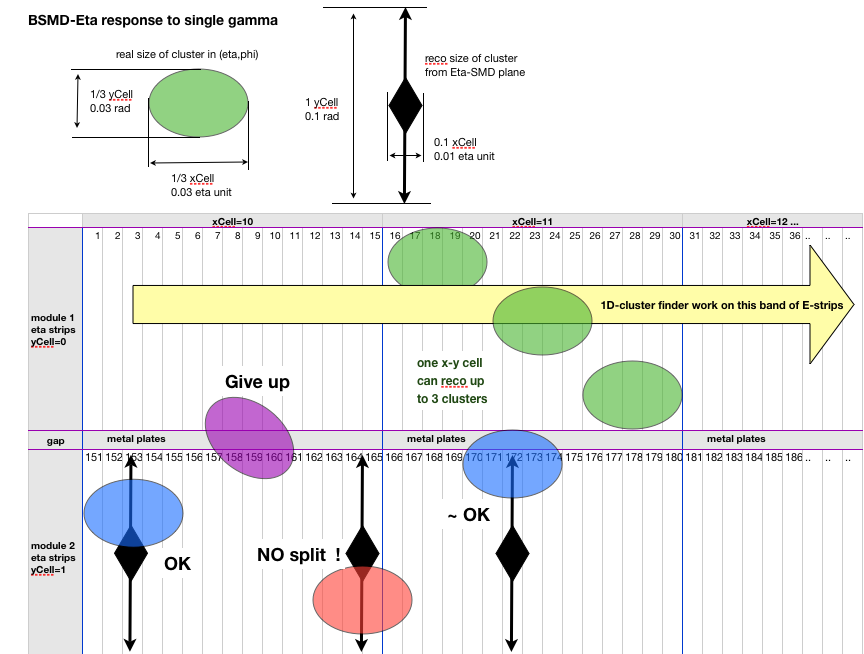
BSMD calibration algo has been developed based on M-C response of BSMD & towers to single gammas.
Executive summary:
The purpose of BSMD absolute calibration summarized at this drupal page is to reconstruct integrated energy deposit (dE) in BSMD based on measured ADC.
By integrated dE in BSMD I mean sum over few strips forming EM cluster, no matter what is the cluster shape.
This calibration method accounts for the varying absorber in front of BSMD and between eta & phi planes.
This calibration will NOT help in reconstruction:
- full energy of EM particle which gets absorbed in BEMC ( shower development after BSMD layer does not matter for this calibration).
- partial energy of hadrons passing or showering in BEMC
- correct for the incident angle of the particle passing through detector
- saturation of BSMD readout. I only state up to which loss (DE) the formula used in reconstruction:
dE/GeV= (rawAdc-ped) * C0 * (1 +/- C1etaBin)
- determine sampling fraction (SF) of BSMD with high accuracy
Below you will find brief description of the algo, side by side comparison of selected plots for M-C and real data, finally PDF with many more plots.
Proposed absolute calibration coefficients are show in table 2.
Part 1
Description of algorithm finding isolated gammas in the Barrel.

Input events
- M-C : single gamma per event, 6 GeV ET, flat in eta, phi covers 3 barrel modules 12,13,14, geometry=y2006
- DATA: BHT0,1,2 triggered pp 2008 events from day 47, total 100K, individual triggers: 44K, 33K, 40K, respectively
events were privately produced w/ zero suppression.
Raw data processing based on muDst
- M-C : BSMD - take geant energy deposit ~100 keV range, towers - take ADC*0.493 to have nominal calibration of 4070 ADC=60 GeV ET.
- Data : BSMD - use private pedestals & status tables for day 47, use custom calibration
use BSMD calibration dE/GeV= (rawAdc-ped) * C0 * (1 +/- C1etaBin), where '+' is for Phi-plane and '-' for eta plane, see table below
skip strips 4 sigma above ped or with energy below 1keV, strip to strip relative gains NOT used , data from CAPs=123,124,125 were not used
towers- take ADC as is, no offline gains correction.
Cluster finder algo (seed is sliding fixed window), tuned on M-C gamma events
- work with 150 Eta-strips per module or 900 Phi-strips at fixed eta
- all strips are marked as 'unused'
- sum dE in fixed window of 4 unused strips, snap at location which maximizes the energy
- if sum below 10 keV STOP searching for clusters in this band
- add energy from one strip on each side, mark all 1+4+1 strips as 'used'
- compute energy weighted cluster position and RMS
- goto 1
This cluster finder process full Barrel West, more details about clustering is in one cluster topology , definition of 'barrel cell'
Isolated EM shower has been selected as follows, tuned on gamma events,
- select isolated eta-cluster in every segment of 15 eta strips.
- require cluster center is at least 3 strips away from edges of this segment (defined by eta values of 0.0, 0.1, 0.2,....0.9, 1.0)
- require there is only one phi-cluster in the same 0.1x0.1 eta.phi cell
- require phi-cluster center is at least 3 strips from the edges
- find hit tower matching to the cross of eta & phi cluster
- sum tower energy from 3x3 patch centered on hit tower
- require 3x3 tower ADC sum >150 ADC (equivalent to 2.2 GeV ET, EM)
- sum tower energy from 5x5 patch centered on hit tower
- require 3x3 sum/ 5x5 sum >0.9
- require RMS of Phi & Eta-cluster is above 0.2 strips
Below is listing of all cuts used by this algo:
  useDbPed=1; // 0= use my private peds
  par_skipSpecCAP=1; // 0 means use all BSMD caps
  par_strWinLen=4; (3)  // length of integration window, total  1+4+1, in strips
  par_strEneThr=1.e-6;  (0.5e-6) // GeV, energy threshold for strip to start cluster search
  par_cluEneThr=10.0e-6; (2.0e-6) // GeV, energy threshold for cluster in window
  par_kSigPed=4.; (3) // ADC threshold
  par_isoRms=0.2;  (0.11) // minimal smd 1D cluster RMS
  par_isoMinT3x3adc=150; //cut off for low tower response
  par_isoTowerEneR=0.9; //  ratio of 3x3/5x4 cluster
(in red are adjusted values for MIP or ET=1GeV cluster selection)
Table 1 Tower cluster cut defines energy of isolated gammas.
| 3x3 tower ET (GeV), trigger used | MIP, BHT0,1,2 | 1.0, BHT0,1,2 |
3.4, BHT0 |
4.7, BHT1 |
5.5, BHT2 |
7, BHT2 |
| 3x3 tower ADC sum range | 15-30 ADC | 50-75 ADC | 170-250 ADC | 250-300 ADC | 300-380 ADC | 400-500 ADC |
| 3x3 energy & RMS (GeV) @ eta=[0.1,0.2] | 0.34 +/- 0.06 | 0.92 +/- 0.11 | 3.1 +/- 0.3 | 4.1 +/- 0.2 | 5.1 +/- 0.3 | 6.6 +/- 0.4 |
| 3x3 energy & RMS (GeV) @ eta=[0.4,0.5] | 0.37 +/- 0.07 | 1.0 +/- 0.11 | 3.4 +/- 0.4 | 4.6 +/- 0.3 | 5.6 +/- 0.4 | 7.3 +/- 0.5 |
| 3x3 energy & RMS (GeV) @ eta=[0.8,0.9] | 0.47 +/- 0.09 | 1.3 +/- 0.16 | 4.3 +/- 0.4 | 5.7 +/- 0.3 | 7.1 +/- 0.5 | 9.3 +/- 0.6 |
Table 2 shows assumed calibration.
Contains relative calibration of eta vs. phi plane, different for M-C vs. data,
and single absolute DATA normalization of the ratio of SMD (Eta+Phi) cluster energy vs. 3x3 tower cluster at eta=0.5 .
Table 3 shows what comes from data & M-C analysis using calibration from table 2.

Part 2
Side by side comparison of M-C and real data.
Fig 2.1 BSMD "Any cluster" properties
TOP : RMS vs. energy, only Eta-plane shown, Phi-plane looks similar
BOTTOM: eta -phi distribution of found clusters. Left is M-C - only 3 modules were 'populated'. Right is data, white bands are masked modules or whole BSMD crate 4

Fig 2.2 Crucial cuts after coincidence & isolation was required for a pair BSMD Eta & Phi clusters
TOP : 3x3 tower energy (black), hit-tower energy (green) , if 3x3 energy below 150 ADC cluster is discarded
BOTTOM: eta dependence of 3x3 cluster energy. M-C has 'funny' calibration - there is no reason for U-shape, Y-value at eta=0.5 is correct by construction.

Fig 2.3 None-essential cuts, left by inertia
TOP : ratio of 3x3 tower energy to 5x5 tower energy , rejected if below 0.9
BOTTOM: RMS of Eta & Phi cluster must be above 0.2, to exclude single strip clusters

Part 3
Examples of relative response of BSMD Eta vs. Phi AFTER calibration above is applied.
I'm showing examples for 3 eta slices of 0.15, 0.55, 0.85 - plots for all eta bins are available as PDF, posted in Table 2 at the end.
The red vertical line marks the target calibration, first 2 columns are aligned by definition, 3rd column is independent measurement confirming calibration for data holds for ~40% lower gamma energy.
Fig 3.1 Phi-cluster vs. Eta cluster for eta range [0.1,0.2]. M-C on the left, data in the middle, right.

Fig 3.2 Phi-cluster vs. Eta cluster for eta range [0.4,0.5]. M-C on the left, data in the middle, right.

Fig 3.3 Phi-cluster vs. Eta cluster for eta range [0.8,0.9]. M-C on the left, data in the middle, right.

Fig 3.4 Phi-cluster vs. Eta cluster for eta range [0.9,1.0]. M-C on the left, data in remaining columns.

Part 4
Absolute response of BSMD (Eta + Phi) vs. 3x3 tower cluster, AFTER calibration above is applied.
I'm showing eta slices [0.4,0.5] used to set absolute scale. The red vertical line marks the target calibration, first 2 columns are aligned by definition, 3rd column is independent measurement for gammas with ~40% lower --> BSMD response is NOT proportional to gamma energy.
Fig 4.1 Phi-cluster vs. Eta cluster for eta range [0.4,0.5]. Only data are shown.

Fig 4.2 Absolute BSMD calibration for eta range [0.0,0.1] (top) and eta range [0.1,0.2] (bottom) . Only data are shown.
Left: Y-axis is BSMD(E+P) cluster energy, y-error is error of the mean; X-axis 3x3 tower cluster energy, x-error is RMS of distribution . Fit (magenta thick) is using only to 4 middle points - I trust them more. The MIP point is too high due to necessary SMD cluster threshold, the 7GeV point has very low stat. There is no artificial point at 0,0. Dashed line is extrapolation of the fit.
Right: only slope param (P1) from the left is used to compute full BSMD Phi & Eta-plane calibration using formulas:
slope P1_Eta=P1/2./(1-C1[xCell])/C0
slope P1_Phi=P1/2./(1+C1[xCell])/C0
Using C1[xCell],C0 from table 2.

Fig 4.3 Absolute BSMD calibration for eta range [0.2,0.3] (top) and eta range [0.3,0.4] (bottom) . Only data are shown, description as above.

Fig 4.4 Absolute BSMD calibration for eta range [0.4,0.5] (top) and eta range [0.5,0.6] (bottom) . Only data are shown, description as above.

Fig 4.5 Absolute BSMD calibration for eta range [0.6,0.7] (top) and eta range [0.7,0.8] (bottom) . Only data are shown, description as above.

Fig 4.6 Absolute BSMD calibration for eta range [0.8,0.9] (top) and eta range [0.9,0.95] (bottom) . Only data are shown, description as above.
I'm showing the last eta bin because it is completely different - I do not understand it at all. It was different on all plots above - just reporting here.

Fig 4.7 Expected BSMD gain dependence on HV, from Oleg document The 2008 working HV=1430 V (same for eta & phi planes) - in the middle of the measured gain curve.

Part 5
Possible extensions of this algo.
- cover also East barrel (for the cross check)
- include vertex correction in projecting SMD cluster to tower (perhaps)
- study energy resolution of eta & phi plane - now I just compensated relative gains but the total BSMD energy is simply sum of both planes
- last eta bin [0.9,1.0] is completely different, e.g. there is no MIP peak in the 2D fig 2.2 - BTOW gain (HV) is factor 2 or more way too high in this 2 bins
Justification: Inspect right plot on figures 4.2,...,4.6, in particular note at what gamma energy the blue line reaches ADC of 1000 counts. Look at this pattern vs. eta bin. On the last plot it should happen at gamma energy of ~5 GeV but in reality it is at ~10 GeV. - crate 4 (unmodified) would have different gains - excluded in this analysis
- Speculation: those multiple peaks in raws BSMD spectra (seen by others) could be correlated with BHT0,1,2 triggers
- Scott suggestion: more detailed study of BSMD saturation could use BSMD cluster location for fiducial cut forcing gamma to be in the tower center and use just the hit tower. This needs more stats. This analysis uses 1 day of data and ends up with just ~100 entries per energy point.
- non-linear BSMD response does not mean we can reco cluster position with accuracy better than 1 strip.
Fig 5.1 BSMD cluster energy vs. eta of the cluster.

Fig 5.2 hit tower to 3x3 cluster energy for accepted clusters. DATA, trigger BHT2, gamma ET~5.5 GeV.

Fig 5.3 hit tower to 3x3 cluster energy for accepted clusters. M-C, single gamma ET=6 GeV, flat in eta .

20 BSMD saturation
The isolated BSMD cluster algo allows to select different range of tower energy cluster as shown in Fig.1
Fig 1. Tower energy spectrum, marked range [1.2,1.8] GeV.

In the analysis 5 energy tower slices were selected: MIP, 1.5 GeV, and around BHT0,1,2 thresholds.
Plots below show example of calibrated BSMD (eta+phi) cluster energy vs. tower cluster energy. (I added point at zero with error as for next point to constrain the fit)
Fig 2. BSMD vs. tower energy for eta of 0.15, 0.55, and 0.85.

I'm concern we are beyond the middle of BSMD dynamic range for ~6 GeV (energy) gammas at eta 0.5. Also one may argue we se already saturation.
If we want BSMD to work up to 40 GeV ET we need to think a lot how to accomplish that.
Below is dump of one event contributing to the last dot on the middle plot. It always help me to think if I see real raw event.
BSMDE
  i=526, smdE-id=6085 rawADC=87.0 ped=71.4  adc=15.6 ene/keV=0.9
  i=527, smdE-id=6086 rawADC=427.0 ped=65.0  adc=362.0 ene/keV=20.0
  i=528, smdE-id=6087 rawADC=814.0 ped=71.8 adc=742.2 ene/keV=41.0
  i=529, smdE-id=6088 rawADC=92.0 ped=66.4  adc=25.6 ene/keV=1.4


BSMDP
  i=422, smdP-id=6086 rawADC=204.0 ped=99.3  adc=104.7 ene/keV=7.8
  i=423, smdP-id=6096 rawADC=375.0 ped=98.5  adc=276.5 ene/keV=20.3
  i=424, smdP-id=6106 rawADC=692.0 ped=100.1  adc=591.9 ene/keV=47.3


2D cluster
bsmdE CL  meanId=6086 rms=0.80 ene/keV=66.80 inTw 1632.or.1612
bsmdP CL  meanId=6106 rms=0.68 ene/keV=75.45 inTw 1631.or.1632

BTOW
  id=1631 rawADC=43.0 ene=0.2 ped=30.0,  adc=13.0
  id=1632 rawADC=401.0 ene=6.9 ped=32.4  adc=368.6
  id=1633 rawADC=43.0 ene=0.1 ped=35.5   adc=7.5

 gotTwId=1632
 gotTwAdc=368.6
tow3x3 sum=405.7 ADC
3x3Tene=7.3GeV
1) M-C : response of BSMD , single particles (Jan)
Below are studies of BSMD response and calibration algo based on BMSD response to single particle M-C
1) BSMD-E clusters, sliding max, fixed width
Goal: study SMDE energy resolution and cluster shape for single particles M-C
Input: single particle per event, fixed ET=6 GeV, flat eta [-0.1,1.1], flat |phi| <5 deg, 500 eve per sample, Geant geometry y2006
Cluster finder algo (sliding fixed window), tuned on electron events
- work with 150 Eta-strips per module
- sum geant dE in fixed window of 4 strips
- maximize the sum, compute energy weighted cluster position and RMS inside the window
- algo quits after first cluster found in given module
Example of BSMDE response for electon:
McEve BSMD-E dump, dE is Geant energy sum from given strip, in GeV
dE=1.61e-06 m=104 e=12 s=1 stripID=15462
dE=2.87e-05 m=104 e=13 s=1 stripID=15463
dE=8.35e-06 m=104 e=14 s=1 stripID=15464
dE=1.4e-06 m=104 e=15 s=1 stripID=15465
ALL plots below have energy in keV , not MeV - I'll not change plots.
Results:
Fig 1. gamma - later, job crashed.
Fig 2. electron

Fig 3. pi0

Fig 4. eta

Fig 5. pi minus

Fig 6. mu minus

2) BSMDE , 1+3+1 sliding cluster finder
Goal: test SMDE cluster finder on single particles M-C
Input: single particle per event, fixed ET=6 GeV, flat eta [-0.1,1.1], flat |phi| <5 deg, 5k eve per sample, Geant geometry y2006
Cluster finder algo (seed is sliding fixed window), tuned on pi0 events
- work with 150 Eta-strips per module
- all strips are marked as 'unused'
- use only module 13, covering ~1/3 of probed phase space
- sum geant dE in fixed window of 3 unused strips, snap at location which maximizes the energy
- if sum below 5 keV STOP searching for clusters in this module
- add energy from one strip on each side, mark all 1+3+1 strips as 'used'
- compute energy weighted cluster position and RMS
- goto 1
Example of BSMDE response for pi0:
...
strID=1932 u=0 ene/keV=0
strID=1933 u=1 ene/keV=0    +
strID=1934 u=1 ene/keV=2.0  *
strID=1935 u=1 ene/keV=48.2 *X
strID=1936 u=1 ene/keV=3.9  *
strID=1937 u=1 ene/keV=0.8  +
strID=1937 u=0 ene/keV=0
strID=1938 u=0 ene/keV=0
strID=1939 u=2 ene/keV=1.5  +
strID=1940 u=2 ene/keV=8.2  *
strID=1941 u=2 ene/keV=28.1 *X
strID=1942 u=2 ene/keV=13.8 *
strID=1943 u=2 ene/keV=4.0  +
strID=1944 u=0 ene/keV=5.6
strID=1945 u=0 ene/keV=0.5
strID=1946 u=0 ene/keV=0
strID=1947 u=0 ene/keV=0
...
| particle | any cluster found in the module, all eventsFig 1a | only events with exactly 2 found clustersFig 1b |
e- |  |  |
| . | Fig 2a | Fig 2b |
pi0 |  |  |
| . | Fig 3a | Fig 3b |
eta |  |  |
3) same algo applied to full East BSMDE,P
Smd cluster finder with sliding window of 3 strips + one strip on each end (total 5 strips) applied to all 9000 BSMDE,P strips, one gamma per event
4) demonstration of absolute calib algo on single particle M-C
Goal: determine absolute calibration of BSMDE,P planes
Method: identify isolated EM shower and match BSMD cluster energy to tower energy
INPUT events: single particle per event, fixed ET=6 GeV, flat eta [-0.1,1.1], flat |phi| <5 deg, 5k eve per sample, Geant geometry y2006
Cluster finder algo (seed is sliding fixed window), tuned on pi0 events
- work with 150 Eta-strips per module or 900 Phi-strips at fixed eta
- all strips are marked as 'unused'
- use only module 13, covering ~1/3 of probed phase space
- sum geant dE in fixed window of 3 unused strips, snap at location which maximizes the energy
- if sum below 5 keV STOP searching for clusters in this module
- add energy from one strip on each side, mark all 1+3+1 strips as 'used'
- compute energy weighted cluster position and RMS
- goto 1
This cluster finder process full Barrel West, more details about clustering is in one cluster topology , definition of 'barrel cell'
Isolated EM shower has been selected as follows, tuned on gamma events,
- select isolated eta-cluster in every segment of 15 eta strips.
- require cluster center is at least 3 strips away from edges of this segment (defined by eta values of 0.0, 0.1, 0.2,....0.9, 1.0)
- require there is only one phi-cluster in the same 0.1x0.1 eta.phi cell
- require phi-cluster center is at least 3 strips from the edges
- find tower matching to the cross of eta & phi cluster
- require this tower has ADC>100
Example of EM cluster passing all those criteria is below:
smdE: ene/keV= 40.6   inTw 451.or.471
 cell(15,12),   jStr=7 in xCell=15
...
id=1731  ene/keV=4.9  *
id=1732  ene/keV=34.3  X *
id=1733  ene/keV=1.5  *
...
---- end of SMDE dump


smdP: ene/keV= 28.5  inTw 471.or.472
  cell(15,12),   jStr=7 in xCell=15
...
id=1746  ene/keV=2.7  *
id=1756  ene/keV=22.0  X *
id=1766  ene/keV=3.7  *
...
---- end of SMDE dump

muDst BTOW
  id=451, m=12 rawADC=12.0
* id=471, m=12 rawADC=643.0
  id=472, m=12 rawADC=90.0
  id=473, m=12 rawADC=10.0
Results for gamma events
will be show with more details. The following PDF files contain full set of plots for all other particles.
particle | # of eve | plots |
| gamma | 25K | |
| e- | 50K | |
| pi0 | 50K | |
| eta | 50K | |
| pi- | 50K |
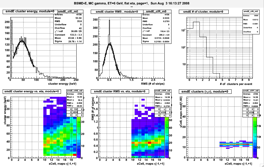
Fig 1, Any Eta-cluster, single gamma, 25K events
TOP: a) Cluster (Geant) energy; b) Cluster RMS, c) # of cluster per event,
BOTTOM: X-axis is eta location, 20 bins span eta [-1,+1]. d) cluster ene vs. eta, e) cluster RMS vs. eta, f) cluster yield vs. eta & phi.

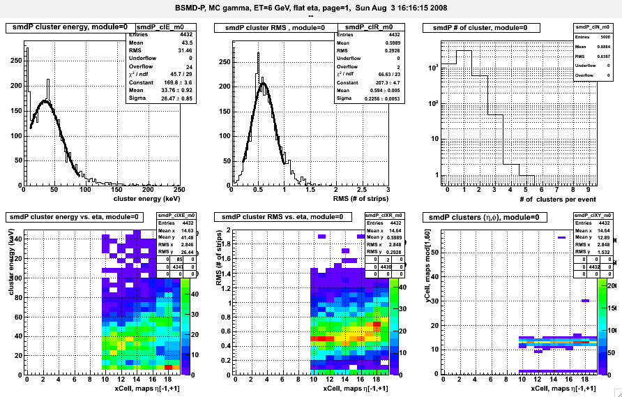
Fig 2, Any Phi-cluster, single gamma, 25K events
see Fig 1 for details

Fig 3, Isolated EM shower, single gamma, 90K events
TOP: a) cluster loss on subsequent cuts, b) # of accepted EM cluster vs. eta location, c) ADC distribution of hit tower (some wired gains are in default M-C), tower ADC is in ET
BOTTOM: X-axis is eta location, 20 bins span eta [-1,+1]. d) Eta-cluster , e) phi-cluster energy, f) hit tower ADC .

Fig 4, Calibration plots, single gamma, 90K events.
TOP: BSMD Eta vs. Phi as function of pseudorapidity. BOTTOM: BSMD vs. BTOW as function of pseudorapidity.3 eta location of 0.1, 0.5, 0.9 of reco EM cluster are shown in 3 panels (2x2)
1D plots are ratios of the respective 2D plots.
The mean values of 1D fits are relative gains of BSMDP/BSMDP and BSMD/BTOW , determine for 10 slice in pseudorapidity. Game is over :).

Fig 5, Same as above, eta=0.1, single pi0, 50K events.

Fig 6, Same as above, eta=0.1, single pi minus, 50K events.

Below are PDF plots for all particles:
Correction - label on the X-axis for 1D plots is not correct. I did not apply log10() - a regular ratio is shown, sorry.
5) Evaluation of BSMD dynamic range needed for the W program at STAR, ver 1.0
M-C study of BSMD response to high energy electrons

Attachment 1:
Fig 1 & 2 reminds actual (pp data based) calibration for 2 eta location of 0.1 and 0.8, presented earlier.
Table 1 shows M-C simulation of average cluster energy (deposit in BSMD plane), its spread, and width as function of electron ET, separately for eta- & phi-planes of BSMD.
As expected, BSMD sampling fraction (SF, red column) is not constant but drops with energy of electron.
The BSMD SF(ET) deviates from constant by less then 20% - it is a small effect.
Fig 3,4,5 show expected BSMD response to M-C electrons with ET of 6,20, and 40 GeV. Only for the lowest energy the majority of EM showers fit in to the dynamic range of BSMD, which ends for energy deposit of about 60 keV per plane.
I was trying to be generous and draw the red line at DE~90 keV .
The rms of BSMD cluster is about 0.5 strips, so majority of energy is measured by just 2 strips (amplifiers). Such narrow cluster lowers saturation threshold.
Fig 6, shows BSMD cluster energy for PYTHIA W-events.
Fig 7 shows similar response to PYTHIA QCD events.
Compare area marked with red oval - there is strong correlation between BSMD energy and electron energy and would be not wise to forgo it in the e/h algo.
Conclusion:
The attached slides show 2008 HV setting of BSMD would lead to full saturation of BSMD response for electrons from W decay with ET as low as 20 GeV , i.e. would reduce BSDM dynamic range to 1 bit.0
For the reference:
* absolute BSMD calibration based on 2008 pp data.
http://drupal.star.bnl.gov/STAR/subsys/bemc/calibrations/bsmd/2008-bsmd-calibration/19-isolated-gamma-algo-description-set-2-0
* current BSMD HV are set very high , leading to saturation of BSMD at gamma energy of 7-10 GeV, depending on eta and plane. (Lets ignore difference between E & ET for this discussion, for now).
http://drupal.star.bnl.gov/STAR/subsys/bemc/calibrations/bsmd/2008-bsmd-calibration/20-bsmd-saturation
* STAR priorities for 2009 pp run presented at Apex: http://www.c-ad.bnl.gov/APEX/APEXWorkshop2008/talks/Dunlop_Star_Apex_2008.pdf
* Attachment 2,3 show BSMD-E, -P response for electrons with ET: 4,6,8,10,20,30,40,50 GeV and to Pythia W, QCD events (in this order)
BSMD 2005 energy scale uncertainty
STAR/blog/ogrebeny/2009/jun/08/bsmd-energy-scale-uncertainty
Definition of absolute BSMD calibration
NOT FINISHED
Definitions of quantities used for empirical calibration of BSMD.
Revised January, 26, 2009
A) Model of the physics process (defines quantities: E, eta, smdE, smdEp, smdEe, C0, C1)
- gamma particle with fixed energy E enters projectively EMC at fixed pseudo-rapidity eta. Eta is defined in detector ref. frame.
- EM showers develops and BSMD (consisting of 2 planes) captures smdEtot of shower energy. Single plane captures smdE=0.5*smdEtot. The SMD cluster energy from single plane is denoted as smdE.
- SMD consist of 2 planes : eta-plane closer to IP and the outer phi-plane. Each plane captures non-equal fraction ofenergy deposited in BSMD: smdEp, smdEe, respectively.
 The following relation holds:
smdEp(E,eta) =smdE(E) * [1-C1(eta)]
smdEe(E,eta) =smdE(E) * [1+C1(eta)]
where theta-dependent coefficient C1 accounts for all physical processes differentiating fraction of captured shower energy by eta vs. phi-planes along Z-direction.
allows reconstruction of full BSMD energy deposit independent on gamma angle theta if cluster energy in both plane is measured - BSMD Cluster energy is measured in each plane by few consecutive strips which:
- response is linear and
- strip-to-strip local hardware gain variation is negligible (the "long-wave" is accounted for in C1(theta))
Note, there are 4 low gain strip (id=50,100) in the eta-plane , seen in fig 2 of 08) SMD-E gain equalization , ver 1.1, which require ADC to be rescaled appropriately.

- The overall conversion constant C0=6.5e-8 (GeV/ADC chan) allows reconstruction of BSMD cluster energy in given plane based on the sum of ADCs from all strips participating in the cluster
smdEp(E,eta)=C0* sum{ ADC_i - ped_i}, over cluster of few strips , similar formula for smdEp(E,eta)=....
The value of C0 was determined based on 19) Absolute BSMD Calibration, table ver2.0, Isolated Gamma Algo description, table 2. Gammas with ET=6 GeV were thrown at EMC and resulting SMD cluster ADC sum was matched to the average value seen for 2008 pp data.
To summarize
The reconstructed cluster energy in each plane with use of C0 & C1 should have eta dependence
smdE(E) =C0* sum{ ADC_i - ped_i}/[1-C1(eta)] for phi-plane cluster
smdE(E) =C0* sum{ ADC_j - ped_j}/[1+C1(eta)] for eta-plane clusterThose 2 quantities are well suited to place cuts.
B) Determination of C1(eta) was based on 19) Absolute BSMD Calibration, table ver2.0, Isolated Gamma Algo description, from crates 1,2,and 4.
Data analysis was done for 10 pseudo-rapidity ranges [0,0.1], [0.1,0.2] ,..., as shown in table 2, row labeled 'DATA'.
For practical application analytical approximation is provided
C1(eta)= C1_0 + C1_1*|eta| + C1_2*eta*eta
symmetric versus positive/negative pseudo-rapidity.
The numerical values of expansion coefficients are: C1_0=0.014, C1_1=0.015, C1_2=0.333
C) Modeling of BSMD response in STAR M-C
- find geantDE geant energy deposit for given BSMD strip
- undo simulated by GEANT +/-7% difference between eta/phi planes (see 19) Absolute BSMD Calibration, table ver2.0, Isolated Gamma Algo description, row 'M-C')
geantDEp=geantDE*0.93
geantDEe=geantDE*1.07 - compute ADC for every i-th strip & plane
ADCp_i= geantDEp/[1-C1(eta)]/C0
ADCe_i= geantDEe/[1+C1(eta)]/C0- If NO saturation is assumed that is all - use ADC-values in reconstruction.
- To simulate full ADC saturation at 1024 assume pedestal is at ADC=100 and saturate values of ADCp_i, ADCe_i at 924. Then proceed to reconstruction.
Mapping, strip to tower distance
For every strip we find the closest tower and determine the distance between tower center and strip center.
Both plots show strip ID on the X-axis, and tower ID on the Y-axis. Error in Y is distance between centers in CM.
It is not true 15 eta strips covers every 2 towers! It is only approximate since strip pitch is constant bimodal and tower width changes continuously.
There is still small problem, namely strip Z is calculated at R_smd and tower Z is calculated at the entrance of the tower
leading to clear paralax error - we are working on this.
Fig 1.
Top plots is for SMDE for module 1. Note E-strip always spans 2 towers and we used tower IDs in one module.
Bottom plots shows phi strips for module 1.

Fig 2.
Top plots is for SMDE for modules 1-4.
Bottom plots shows phi strips for modules 1-4.


Run 10 BSMD Calibrations
Parent page for BSMD Run 10 Calibration
BSMD Status Table in run10 AuAu200GeV runs
==========
We started this task by looking at BSMD in Run 10 with some MuDst files, and found the pedestals probably need to be QA-ed as well.
http://www.star.bnl.gov/HyperNews-star/get/emc2/3500.html
and
http://www.star.bnl.gov/HyperNews-star/get/emc2/3515.html
==========
Then we started to look for Non-zero-suppressed BSMD data, and found that we have to run through the daq files to produce the NZS data files to produce the NZS data. The daq files are stored on HPSS, and we have to transfer them onto RCF. The transferred daq files were then made into root files with Willim's BSMD online monitering codes.
http://www.star.bnl.gov/HyperNews-star/get/emc2/3533.html
==========
We decided to use same critiria and status codes as Willim used for run09 pp500GeV.
http://drupal.star.bnl.gov/STAR/blog-entry/wleight/2009/may/13/bsmd-status-cuts-and-parameters
==========
We discovered that a modification is needed to the critiria of code bit 3 (the ratio of the integral over a window to the integral over all, i.e. the pedestal integral ratio) We found about half of the BSMD strips fail the criteria of this ratio > 0.95, but nearly most of them satisfy ratio > 0.90, so the critiria is loosed to 0.90. We think this is a reasonable difference between run09 pp and run10 AuAu collisions.
http://www.star.bnl.gov/HyperNews-star/get/emc2/3546/1/1.html
==========
The daq files are huge in size, on the order of TB for one day. In order to not disturb the run10 data production, we had to only copy 1/10~1/20 of the daq files.
http://www.star.bnl.gov/HyperNews-star/get/emc2/3589/2.html
==========
After a long period of transffering and root files making, almost all the days between Jan/02/2010 and Mar/17/2010 are done.
http://www.star.bnl.gov/HyperNews-star/get/emc2/3601.html
We found that another criteria has to be modified, because we use NZS data for the QA of the tail of ADC spectrum. The definition of the tail ranges and the limits are adjusted. Three ranges of the tail part of ADC are defined,
Range 1:peak+6*rms to peak+6*rms+50 channels
Range 2:6*rms+50 channels to 6*rms+150 channels
Range 3:6*rms+150 channels to 6*rms+350 channels
The entries (hits) in these three ranges are counted, and the ratios to all the entries in the whole spectrum are calculated. The limits for good ratios are selected based on the ratios distribution trough out all the days. They are
@font-face {
font-family: "Cambria";
}p.MsoNormal, li.MsoNormal, div.MsoNormal { margin: 0in 0in 0.0001pt; font-size: 12pt; font-family: "Times New Roman"; }div.Section1 { page: Section1; }
Range 1: 3.35~80 x0.001
Range 2: 0.95~40 x0.001
Range 3: 0.25 ~ 20 x0.001
See the attached newlimits.docx for more details and plots.
Also, bit 0 of the status code is supposed to indicate whether a channel is bad or not. Not every problem is fatal, i.e cause the channel to be regarded as bad.
Originally, only if all the 3 ratios are beyond the limits, a fetal condition is met; we addjusted this to be if more than one, i.e. >=2, out of the 3 ratios are beyond the limits, a fetal condition is met. One can also treat any channel with a code not equal to 1 as bad, regardless what the bit 0 is.
==========
A final report with sample codes in one day was presented to and approved by EMC2 group.
http://www.star.bnl.gov/HyperNews-star/get/emc2/3637/1.html
==========
Note: The map file used in bsmd montoring in run10 was with some inconsistence with the acctual hardware. An after-burn map correction was done by the EMC software coordinator, Justin.
Note: Up to now, no corrections are made to pedestals. The bad strips caused by bad pedestals are rouphly 1/3~1/4 of all the bad strips.
Wenqin Xu
16Feb2011
Run 9 BSMD Calibration
Parent page for BSMD Run 9 Calibration
01 Status of BSMDE,P at the end of pp 500 GeV run, April of 2009
Summary of BSMD performance on April 6. Input : 200K events tagged by L2W clust ET>13 GeV, days 85-94, ~all events, only ZS data are shown.


Attached PDFs shows zoom in spectra for individual modules. 1st page is summary, next I show 3 modules per row, 5 rows per page. Even pages shows zoom-in for low ADC<100, odd pages shows full ADC scale. Common maxZ=1000 is used for all plots , except page 1.
02 offline QA of BSMD pp 500, ver1 (Willie+Jan)
BSMD QA algorithm and results for pp 500, tune optimized for high energy energy response
- QA method, details are given in Willie's blog
Fig 1. Typical good/bad strips from the E-plane and with wide pedestals.

- Input: all available events from fills 10399, 10402, 10403, 10404, 10407, 10412, 10415 added together
- evaluate shape of pedestal residua for NZS data captured on-line by Willie's daq reader (Blue filled histo)
- evaluate yield in high energy range (ADC ~300,500,800) using ZS data from L2W triggered events (Magenta line-only)
- ignored: satellite spikes around pedestal at ADC ~32, those come from correlated noise and (most likely) such events will be discarded.
- Example of such spectra for few strips is shown in fig 1.
- Encoding of BSMD status bits extends existing convention to use LSB=1 for good strips and LSB=0 for bad strips. We used bits 1,2,3 to tag pedestal problems and bits 5,6,7 to tag yield problems.
- More plots with individual strips is in attachment A,B,C,D.
- Bad strip is defined as having : bad pedestal or god pedestal but no yield above it.
Fig 2. Distribution of bad strips from both planes, details about each plane separately is in attachment E.

- The remaining issues:
- of tagging 'spiked' events (or modules?) needs to be investigated.
- study time dependence
- For the reference this directory contains PDF files with plots from all 120 BSMD modules.
Fig 3. # of bad strips per module.

03 correlated, small ADC spikes in BSMD (Jan)
Study of small ADC spikes in BSMD
Input:
The following plots support those observation:
- spikes are symmetric on both sides of pedestals peak, separated by 2^N ADC counts, narrower than pedestal peak, (Fig1)
- spikes are correlated in even ID (or odd) strips the same plane, correlation is local, Fig 2
- spikes are correlated between P-plane & E-plane strips, Fig 3
- energy deposit in BSMD increases probability of spikes, see peak/valley for blue vs. magenta in fig 1b.
- bands are visible at larger ADC, as shown by Oleg, not sure what data and how many events, fig 4
- perhaps fig 1c shows yet another pathology, because it does not obey odd/even rule in fig 1a & 1b.
Fig 1a. Example of spikes delADC=16, in the vicinity of strip 1525-P, all strips from module 11 are shown in attachment A.

Fig 1b. Example of spikes delADC=32, in the vicinity of strip 1977-P, all strips from module 14 are shown in attachment B, module 22 looks similar.

Fig 1c. Example of spikes delADC=128, in the vicinity of strip 4562-P, all strips from module 31 are shown in attachment C, modules 51,52,57 look similar

Fig 2. Phi-Phi plane correlation of P-strip 1979 with (odd) P-strips: 1977..1994. Attachment D contains correlation of P-strips [1977-80] with 24 strips in proximity.

Fig 3. Phi-Eta plane correlation of P-strip 1979 with (odd) E-strips: 1977..1994. Attachment E contains correlation of P-strips [1977-80] with 24 strips in proximity.

Fig 4.Oleg observed this stripes in raw BSMD ADC spectrum, not sure what data.

2009 BSMD Relative Gains Information
The pdf posted here has a good overview of the computation of the slope for each strip, discussing the method and the various ways in which strips were marked as bad. This page discusses the computation of the actual relative gains and statuses that went into the database.
The code used to compute the relative gains is archived at /star/institutions/mit/wleight/archive/bsmdRelGains2009/.
DELETE - Run 9 BSMD Status Update 3 (4/24)
After looking more closely at the crate 1 channels I was forced to make serious revisions to status bit 2 from the previous update. The new status bit 2 test is as follows:
First, I scan through the strip ADC distribution looking for peaks. A peak is defined as a channel that is greater than or equal to the four or two channels to either side (if the sigma of the fit to the strip ADC distribution is greater than or less than six, respectively), has a content that is greater than 5% of the maximum of the strip ADC distribution, and has a depth greater than 5% of the maximum of the strip ADC distribution. The depth is calculated by first calculating the difference between the peak content and the channel content for each of the four or two channels on either side of the peak. The maximum of these differences is obtained for the left and right sides separately, and the depth is then equal to the lesser of these two maxima.
If the strip has more than one peak and the maximum of the depths is greater than 20% of the maximum of the strip ADC distribution, then the strip is given bad status 2. If the strip has only one peak (which is then necessarily the maximum of the entire distribution) but the distance between that peak and the peak obtained from the gaussian fit is greater than 75% of the sigma from the gaussian fit, the strip is given bad status 2 as well. Attached is a pdf that has only the pedestal plots for all channels from crate 1.
Edit: I forgot that the BSMD crates don't increase with module number: what is labeled as crate 1 is actually crate 2, as that is the crate that has the first 15 modules, and the attachment labeled as crate 2 is the 2nd 15 modules and so actually crate 1.
2nd edit: This is now out of date, please see the new update.
DELETE - Run 9 BSMD Status Update 4 (4/27)
After further investigations -- specifically looking at strips that had a significant secondary peak, entirely separated from the main peak, with a max of ~40, which were not being caught by my cuts -- I have again revised my criteria for status bit 2. Again, I begin by looking for peaks. If a peak candidate is less than three sigma from the peak of the strip ADC distribution (strip and peak both taken from the gaussian fit), the same cuts are imposed: the candidate must be greater than the four (if sigma>6) or two (if sigma<6) channels on on either side of it, it's content must be greater than 5% of the maximum of the strip ADC distribution, and the depth must be at least 5% of the maximum of the strip ADC distribution. If the strip has two such peaks with the maximum of the depths greater than 20% of the maximum of the strip ADC distribution, or has only one peak but that peak is at least one sigma away from gaussian fit peak, it is given bad status 2. Note the only change here is that the previously a strip with only one peak could be marked bad if it was 75% of sigma away from the gaussian fit peak.
Most of the changes have to do with candidates that are at least three sigma from the gaussian fit peak. In this case the cuts are relaxed: the bin content need only be .5% of the max, not 5%, though it still must be at least 10, and the peak depth is required to only be at least 5% of the peak itself, not of the max. A more than three-sigma peak has the same requirements for the number of channels it must be greater than: however, none of those channels can have value 0. Any strip with a candidate that passes these criteria is automatically given bad status 2.
Pdfs for crates 1 and 2 are attached (but note that the crate 1 and crate 2 pdfs contain the first and second 15 modules, respectively, and therefore crate 1 should actually be labeled crate 2 and crate 2 is really crate 4).
DELETE - Run 9 BSMD Status Update 5 (4/30)
Edited on 5/1 to reflecte new status bit assigments for bits 3 and 4.
The current BSMD status bits are as follows:
Bit 2: Bad pedestal peak/multiple pedestal peaks. This is described in more detail here. Examples can be found in crate2_ped.pdf pp 207 and 314 and crate4_ped.pdf p 133.
Bit 3: Pedestal peak has bad sigma, sigma<1 or sigma >15
Bit 4: Chi squared value from gaussian fit is greater than 1000 (i.e., pedestal has a funny shape)
Bit 5: Strip is exactly identical to the previous strip
Bit 6: The ratio of the integral of channels 300-500 to the total integral does not fall between .0001 and .02
Bit 7: The ratio of the integral of channels 500-800 to the total integral does not fall between .00004 and .02
Bit 8: The ratio of the integral of channels greater than 800 to the total integral does not fall between .00005 and .02
Note that this means that dead channels have status 111xxxx0->448 (or greater).
The attached pdfs crate2 and crate4.pdf have the pedestal distributions, taken from NZS data, and the overall distributions, taken from ZS L2W data, overlayed; crate2_ped and crate4_ped.pdf have only the pedestal distributions. The NZS data used was taken from my monitoring for fills 10415-10489. The L2W data came from fills 10383-10507. Additionally, at the beginning of each module is a summary page that has plotted the distributions for the ratios used to determine bad status bits 6, 7, and 8, and the overal distribution of status vs. strip for eta and phi.
Finally, there are a couple of possible new problems. Page 18 in crate4_ped.pdf has several examples of pedestal distributions that have shoulders. Page 20 has a few examples of pedestal distributions with a small, skinny peak perched on top of a large, broad distribution. At the moment I have no bad status bit for either of these, and any peak with either of these features would almost certainly not be marked bad (even though I did manage to catch one of the ones on page 20).
Edit: Scott suggested during the phone meeting today that perhaps the problem of a small peak on a broad distribution was due to time variation of the pedestal width, and in the plot below you can see that he was correct: the strip initially has an extremely wide pedestal which then shrinks down suddenly. Futhermore, looking at one of the strips that had a sort of shoulder to it, you can see that this is just a less-pronounced version of the double peak problem seen before: the pedestal goes up by 10 for a much shorter time frame, thus producing a shoulder rather than a second peak. This suggests that, as Scott said, these channels should still be usable, and that once we begin breaking status down by time these funny shapes should be less of a problem.


DELETE - Run 9 BSMD Status Update 6 (5/4)
As Matt says that the maximum status is 255, I have dropped the old status bit 5 as (it was unused). Also, I have loosened the dead strip cuts based on looking at module 55 (see pages 203 or 205 in the attached crate1.pdf, for instance). The status bits are now as follows:
Bit 2: Bad pedestal peak/multiple pedestal peaks.
Bit 3: Pedestal peak has bad sigma, sigma<1 or sigma >15
Bit 4: Chi squared value from gaussian fit is greater than 1000 (this applies only for strips that do not have bad status 2 already)
Bit 5: The ratio of the integral of channels 300-500 to the total integral does not fall between .0005 and .02
Bit 6: The ratio of the integral of channels 500-800 to the total integral does not fall between .0002 and .02
Bit 7: The ratio of the integral of channels greater than 800 to the total integral does not fall between .0002 and .02
Below is a plot of status vs. eta and phi for BSMDE and BSMDP strips. Note that strips with all three of bits 5, 6, 7 bad (generally, dead strips) are given the value 8 in this plot to distinguish them from strips that may have just one of those bits bad. As some strips may have more than one bad status bit, for clarity I ranked the potential bad statuses in the order 2, 8, 7, 6, 5, 4, 3 (i.e., approximately in order of importance) and plotted for each strip only the highest-ranked status.

Additionally, I found a problem I had not seen before. On page 207 of the attached crate1.pdf you can see that in the L2W data some strips have a large peak out in the tail of the ADC distribution. However, as all these strips are caught by my code it's not a serious problem.
Final Run 9 200 GeV BSMD Status
In essence, the 200 GeV status tables were calculated the same way as the 500 GeV tables were. Please see here for details.
Final Run 9 500 GeV BSMD Status - Willie Leight
BSMD Pedestals and Status for Run 9 pp 500 Data (June 2009, uploaded to offline DB)
The BSMD status analysis for the 500 GeV data proceeds as follows:
- Each strip is assigned a status for the whole run from an analysis of fills 10399, 10402, 10403, 10404, 10407, 10412, and 10415. Pedestals are analyzed using NZS data taken by the BSMD online monitoring, which reads NZS data from evp and subtracts off pedestals which are updated each time a new BSMD pedestal run is taken. Because NZS data is essentially minbias, high energy tails are analyzed using L2W-triggered data. Status bits are described in detail here.
- Once each strip has an assigned status, those strips that are not marked as bad move on to the second step. Here the strips are examined fill-by-fill: for each fill the strip pedestal is QAed by re-applying the pedestal cuts (but not the tail cuts due to lack of statistics), and a new status for that fill is determined.
- Next, a pedestal correction is calculated. The pedestal correction is just the MPV of the pedestal residua if the MPV is greater than the RMS of the pedestal residua.
- Finally, we upload a number of tables to the database: for each BSMD plane there is one that contains a universal status for every strip, one for each fill containing a status for every strip, and one for each fill containing the RMS and pedestal correction for every strip.
Attached is a pdf that presents the results of this study, including examples.
All code and root files are archived at /star/institutions/mit/wleight/archive/2009-pp500-bsmdStatus/.
Table 1: Pedestal correction, RMS, and status vs. fill for each module (Crates 1-4 are the West Barrel)
Table 2: BSMD spectra for 150 eta and 150 phi strips used for status determination for each module (for fills listed above). Bad strips are identified with the status (in hex): strips with red status are marked bad, strips with green failed a cut but are not necessarily bad. Note that these spectra are shifted up by 100 on the X-axis so that the pedestal is centered around 100 rather than 0.
Table 3: Fills used in this study.
# Fill Date Begin run End run LT/pb
1 F10383 2009-03-18 R10076134 R10076161 0.00
2 F10398 2009-03-20 R10078076 R10079017 0.08
3 F10399 2009-03-20 R10079027 R10079086 0.22
4 F10402 2009-03-21 R10079129 R10079139 0.04
5 F10403 2009-03-21 R10080019 R10080022 0.01
6 F10404 2009-03-22 R10080039 R10080081 0.09
7 F10407 2009-03-22 R10081007 R10081056 0.05
8 F10412 2009-03-23 R10081096 R10082095 0.23
9 F10415 2009-03-24 R10083013 R10083058 0.24
10 F10426 2009-03-25 R10084005 R10084024 0.11
11 F10434 2009-03-26 R10085016 R10085039 0.18
12 F10439 2009-03-27 R10085096 R10086046 0.26
13 F10448 2009-03-28 R10087001 R10087041 0.29
14 F10449 2009-03-28 R10087051 R10087097 0.32
15 F10450 2009-03-29 R10087110 R10088036 0.29*
16 F10454 2009-03-29 R10088058 R10088085 0.15*
17 F10455 2009-03-30 R10088096 R10089023 0.29*
18 F10463 2009-03-31 R10089079 R10090027 0.20*
19 F10464 2009-03-31 R10090037 R10090047 0.08*
20 F10465 2009-03-31 R10090071 R10090112 0.13*
21 F10471 2009-04-02 R10091089 R10092050 0.30
22 F10476 2009-04-03 R10092084 R10093036 0.28
23 F10478 2009-04-03 R10093057 R10093085 0.08
24 F10482 2009-04-04 R10093110 R10094024 0.55
25 F10486 2009-04-05 R10094063 R10094099 0.52
26 F10490 2009-04-05 R10095019 R10095057 0.40
27 F10494 2009-04-06 R10095120 R10096027 0.61
28 F10505 2009-04-07 R10096139 R10097045 0.39
29 F10507 2009-04-08 R10097086 R10097153 0.29
30 F10508 2009-04-08 R10098029 R10098046 0.17
31 F10517 2009-04-09 R10099020 R10099078 0.32**
32 F10525 2009-04-10 R10099185 R10100032 0.68
33 F10526 2009-04-10 R10100049 R10100098 0.37
34 F10527 2009-04-11 R10100164 R10101020 0.82
35 F10528 2009-04-11 R10101028 R10101040 0.31
36 F10531 2009-04-12 R10101059 R10102003 0.86
37 F10532 2009-04-12 R10102031 R10102070 0.76
38 F10535 2009-04-13 R10102094 R10103018 0.86
39 F10536 2009-04-13 R10103027 R10103046 0.43
* Crate 2 was off for this fill
** This fill had no BSMD data
Final Run 9 BSMD Absolute Calibration
The Run 9 BSMD absolute calibration was made using few-GeV TPC-identified electrons from pp500 running, and has two pieces. The first is a new CALIBRATION table in the database which will be used in the EMC slow simulator to improve the agreement of of MC ADC with data. This table starts by combining the previously-determined strip-by-strip relative gains with the existing values in the table. This is then multiplied by the ratio of the slope of a linear fit to the mean cluster ADC distribution from few-GeV isolated data electrons to the same slope in simulated electrons, where the slope is calculated in four different eta bins. The second piece is a new GAIN table in the database which allows ADC values to be converted to energy deposited in the BSMD. This table was determined by combining the strip-by-strip relative gains with a similar ratio as above, but using mean cluster energy deposited in the BSMD instead of reconstructed ADC values (the electron samples used for data and MC were the same) and it is calculated in ten eta bins instead of four. Both tables are currently in the database with flavor "Wbose2": it is hoped that eventually the CALIBRATION table will migrate to flavor "ofl", but the GAIN table will have to remain "Wbose2" because it is currently used (with values all equal to 1) in some codes to determine the change in the BSMD calibration over time. While producing two tables which are in some ways overlapping and one of which can never be flavor "ofl" is not an ideal solution, it allows us to avoid making any modifications to currently existing code (in particular the StEmcSimulator) and allows people who prefer to think of reconstructed energy from BSMD ADCs as being the full particle energy instead of the energy deposited in the BSMD to continue as they were with no change. For more details, please see:
2. Final cut list and data-MC comparison
Additionally, a link to the 2009 BSMD Calibration note will be added here once it is completed.
See also a brief presentation on why we chose not to include the BSMD gas pressure in our analysis.
Run 9 BSMD Status Update 1 (4/19)
I use two datasets to QA BSMD channels: zero-suppressed data from L2W events (fills 10383-10507) and non-zero-suppressed data from online monitoring (fills 10436-10507) (note that at the moment I am not examining the time dependence of BSMD status). NZS data is used to QA the pedestal peak of a channel, while high-energy ZS data is used to QA the tail.
Next, the ZS data are compared to the ZS data from the previous channel to check for copycat channels. Then three quantities are calculated: the ratios of the integrals from 300-500, 500-800, and 800-the end of the spectrum to the total integral of the channel. Each of these quantities must then fall within the following cuts: .0001-.02, .00004-.02, and .00005-.02 respectively. Here is a sample distribution:

Also, the spectra for the strips in module 3, with status, are attached. I have not had a chance to look closely at any other modules yet.
details about known hardware problems
Attached file 'SMD_07.xls' contain my notes from run 7, the only things that might be useful for
you is in the red color, permanently disconnected anode wires and affected
strips (again this is not SoftIds). I think that I cut out one more wire
before Run8 started, but for that I need to check logbook.
Oleg
-----------------------
BSMD Wire Support Effects on GAIN
Here is a note from Oleg Tsai (and attached file "wiresup.pdf" below) concerning source
measurements of the BSMD gain behavior near the nylon wire supports:
On Fri, 18 Jul 2008, tsai@physics.ucla.edu wrote:
> Attached plot will help you to understand what you see close to
> strips 58 and 105. There are two nylon wire supports in the chamber
> at distances 34.882" and 69.213" from the (eta=0 end of the chamber,
> not from the real eta 0). Gain drops near these supports. You can
> see this in your plots also. The attached plot shows counting rate vs
> strip id for a typical chamber. Don't pay attention to channels
> near 0 and 150 - these effects are due to particular way co60 source
> was collimated (counting profile was close to 0.1/0.2/0.4/0.2/0.1)
> 0.4 in central strip. From that I estimated that eta strips
> 56-60 and 104-107 should have calib. coefficients
> (.95,.813,.875,.971,.984) (.99,.89,.84,.970.), I don't remember
> if I was using counting rate vs HV to derive these numbers...
> (this is my third and final attempt :-))
>
details of SMD simulator, simu shower zoom-in
Fig 1. Geant simu of EM shower of one electron with ET=10 GeV at eta=0.
Note,
- one phi-strip is parallel to cavities, extends over 1/10 of the cavity length, and integrates over 2 consecutive cavities.
- one eta-strip is perpendicular to cavities, extends over 1/150 of the cavity length, and integrates over all 30 cavities in the module.

Hi Jan,
the only documentation I know of is the code itself --
hopefully you'll consider it human-readable. Look at
StEmcSimpleSimulator::makeRawHit() in StEmcSimulatorMaker. We use the
kSimpleMode case. The GEANT energy deposition is multiplied by a
sampling fraction that's a second-order polynomial in pseudorapidity,
and then we take pedestals, calibration jitter, etc. into account.
The exact parameters of the sampling fraction are defined in the
constructor for StEmcSimpleSimulator. I don't remember how they were
determined.
also meant to add that the width broadening is OFF by
default. To turn it on one needs to do
emcSim->setMaxCrossTalkPercentage(kBarrelEtaStripId, aNumber);
The "width broadening" only occurs
for eta strips and was implemented by Mike Betancourt in
StEmcSimulatorMaker::makeCrossTalk(). He wrote a blog post about it:
http://drupal.star.bnl.gov/STAR/blog-entry/betan/2007/nov/19/cross-talk-bsmd
Adam
Maybe I should note that the cross talk I implemented was to account
for the capacitive cross talk between the cables carrying the eta
strip signals to the readout, and not for any effects related to the
energy deposition.
-Mike
Hi Jan,
Well, Oleg should probably make the definitive reply, but I think it is like this:
The amplification happens only at the wire, it is independent of the positions of the primary ionization. Of course, there is a little effect from a small amount of recombination or capture of the charge on impurities, and there must be a (hopefully small) effect from the dependence of the mean pulse shape on the position of the ionization and the dependence of the effective gain of the electronics on the mean pulse shape. But these things can't amount to much, I would think. (Of course, I don't want to discourage you from looking in the data to confirm it!)
Gerard
These are all quite true, small effects which will be difficult
to see. The bigger effect is reading out one time bucket.
I have made some estimates before test run 98 (?) or so, see this PS
if you look at numbers still very small effect which is unpractical
to measure.
Oleg
Hi, Yes indeed, I don't know why I neglected to think of the simple effect of drift time, but it is certainly going to be a much bigger effect (~10% if I read your fig.3 correctly?) than the other two. (Perhaps still too small to see in the data, I don't know...). Anyway, given the data volume and already limited readout speed of the BSMD I am pretty sure there is no prospect to ever read more than the one fixed time sample from BSMD; this is probably something to live with. [But it is not impossible to have 2 or 3 point readout, and if we want to seriously consider it it should be brought up ~now, well that is in case we are given the green light to work on BSMD readout "mini-upgrade". If not, well it will just wait until then. But keep in mind, more points readout would offer slightly better gain accuracy but will complicate offline and calibrations too, probably you really don't want it anyway!]
Gerard
p.s. Jan I don't know if it adds anything to the wider discussion on BSMD gain/cal but if you feel so you may surely post to hn.
p.p.s. Oleg, an important question - in your note you don't specify exactly how you obtain the drift time... I mean, yes you show a drift velocity curve, but really of course you must mean there was a calculation such as with garfield to get a drift time out of this... _So_, was that calculation done with the magnetic field on? [The wires are parallel to the magnetic field, right? So it will make possibly a very big difference in drift times.] Jan, do you/others realize the BSMD gain will probably have some systematic dependence on the magnetic field, including the sign thereof? So if you care about gain calibration it should be separated out according to the state of STAR magnet, fortunately there are only a few running states, right?
Gerard
one cluster topology , definition of 'barrel cell'
One dimensional BSMD cluster finder is insensitive to single dead strips and module boundaries for the phi strip.
However certain class of Phi-strip clusters (marked as red) are artificial split and reco as 2 phi-clusters.
One could use the Eta-strip cluster to recover from such phi-plane split if occupancy is low and relative scale of eta & phi cluster energy known.
Plots below also introduce a concept of 'barrel cell' which has approximate size of 0.1 in eta & phi physical units and is aligned with barrel modules. 'barrel cell' is the smallest common unit in eta-phi space for SMD and BTOW tower topologies.
'Barrel cell' has 2 coordinates : x[0,19] and y[0,59] . If such object is already defined for the Barrel, uniform for East & West let me know and I'll adjust numbering scheme.
Back to recovery of split phi cluster, shown below as red oval. Green clusters are shown to 'calibrate' yourself to this type of representation.
Fig 1.
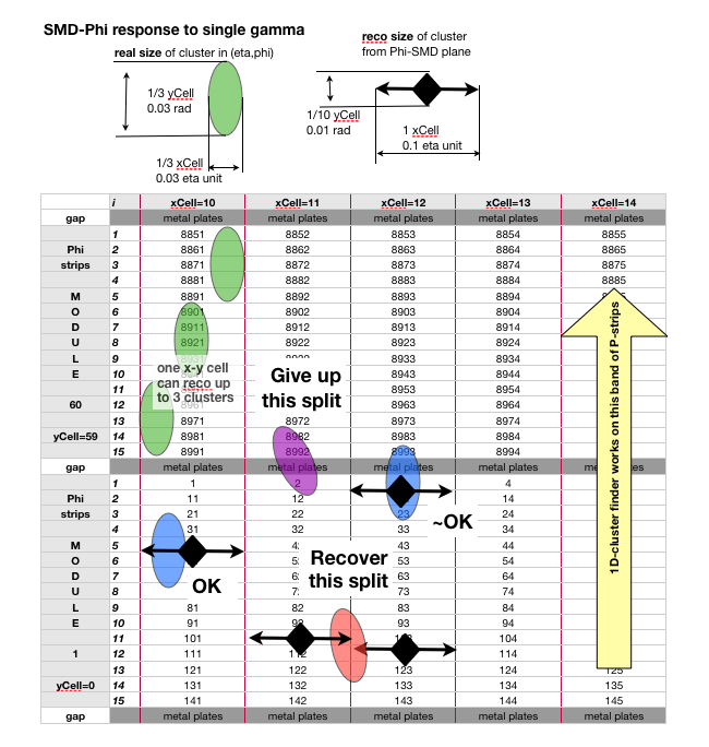
Fig 2.