Run 9 BTOW Calibration
Parent page for BTOW 2009 Calibrations
01 BTOW HV Mapping
We started at the beginning of the run to verify the mapping between the HV cell Id and the softId it corresponds to. To begin, Stephen took 7 runs with all towers at 300V below nominal voltage except for softId % 7 == i, where i was different for each run. Here are the runs that were used:
| softId%7 | Run Number | Events |
| 1 | 10062047 | 31k |
| 2 | 10062048 | 50k |
| 3 | 10062049 | 50k |
| 4 | 10062050 | 50k |
| 5 | 10062051 | 50k |
| 6 | 10062060 | 100k |
| 0 | 10062061 | 100k |
We used the attached file 2009_i0.txt (converted to csv) as the HV file. This file uses the voltages from 2008 and has swaps from 2007 applied. Swaps indentified were not applied and will be used to verify the map check.
File 2009_i0c.txt contains some swaps identified by the analysis of these runs.
File 2009_i1c.txt contains adjusted HV settings based on the electron/mip analysis with same mapping as 2009_i0c.txt.
Final 2009 BTOW HV set on March 14=day=73, Run 10073039 , HV file: 2009_i2d.csv
02 Comparing 2007, 2008 and 2009 BTOW Slopes
We have taken two sets of 1M pp events at sqrt(s)=500 GeV. For future reference, the statistical error on the slopes is typically in the range of 3.7%. I give a plot of the relative errors in the 5th attachment.
plus we have
Comparing the overall uniformity of the gain settings, I give the distribution of slopes divided by the average over the region |ETA|<0.8 for 2007, 2008 and 2009 (First three attachments)
I find that there is little difference in the overall uniformity of the slopes distribution over the detector...about +/-5%. I also give a plot showing the average slopes in each eta ring for the three different voltage settings in each year 2007. 2008 and 2009. (4th attachment) As you can see, the outer eta rings were overcorrected in 2008. They are now back to nearly the same positions as in 2007.
_________________________________________________________________
Here is my measurement of 'kappa' from 2007 data. I get from 7-8, depending on how stringent the cuts are. I think this method of determining kappa is dependent on the ADC fitting range. In theory, we should approach kappa~10.6 as we converge to smaller voltage shifts.
So which ones should we adjust? Here is a fit of the slope distribution to a gaussian.
As we can see, the distribution has an excess of towers with slopes >+/-20% from the average. I checked that these problem towers are not overwhelmingly swapped towers (15/114 outliers are swapped towers; 191/4712 are swapped towers). Here is an eta:phi distribution (phi is SoftId/20%120, NOT angle!). The graph on the left gives ALL outliers, the graph on the right gives outliers with high slopes only (low voltage). There are slightly more than expected in the eta~1 ring, indicating that the voltages for this ring are set to accept few particles than the center of the barrel.
______________________________________________________________________
So Oleg Tsai and I propose to change only those outliers which satisfy the criteria:
|slope/ave_slope - 1|>0.2 && |eta|<0.8. (Total of 84 tubes)
We then looked one-by-one thru the spectra for all these tubes (Run 10066010) and found 12 tubes (not 13 as I stated in my email) with strange spectra:
Bad ADC Channels: Mask HV to Zero
We then calculated the proposed changes to the 2009_i1c.csv HV using the exponent kappa=5. Direct inspection of the spectra made us feel as though the predicted voltage changes were too large, so we recomputed them using kappa=10.48. We give a file containing a summary of these changes:
Proposed HV Changes (SoftId SwappedID Slope(i1c) Ave Slope Voltage(i1c) New Voltage
(We have identified 3 extra tubes with |eta|>0.8 which were masked out of the HT trigger to make it cleaner....we propose to add them to list to make a total of 87-7 = 80 HV changes.)
PS. We would also like to add SoftId-3017 HV800 -> 650. This make 81 HV changes.
_____________________________________________________________________
A word about stability of the PMT High Voltage and these measurements. I compared several pairs of measurements in 2007 taken days apart. Here is an intercomparison of 3 measurements (4,5 and 7) taken in 2007. The slopes have a statistical accuracy of 1.4%, so the distribution of the ratio of the two measurements should have a width of sqrt(2)*1.4 = 2% The comparison of the two measurements is just what we expect from the statistical accuracy of the slope measurements.
Comparing the two recent measurements in 2009, we have a set of about 600 tubes with a very small voltage change. The slopes were measured with an accuracy of 3.7%, so the width of the slope ratio distribution should be sqrt(2)*3.7% =5.2%. Again, this is exactly what we see. I do not find any evidence that (a large percentage of) the voltages are unstable!
___________________________________________________________________
03 study of 2009 slopes (jan)
Purpose of this study is to evaluate how successful was our firts attempt to compute new 2009 HV for BTOW.
Short answer: we undershoot by a factor of 2 in HV power- see fig 4 left.
Input runs: 10066160 (new HV) and 10066163 (old HV)
Fig 1. Pedestal distribution and difference of peds between runs - perfect. Peds are stable, we can use the same slope fit range (ped+20,ped+60) blindly for old & new HV.

Fig 2. Chosen HV change and resulting ratio of slopes - we got the sign of HV change correctly!

Fig 3. Stability test. Plots as in fig 2, but for a subset of towers we change HV almost nothing (below 2V) but yield was large. One would hope slope stay put. They don't. This means either slopes are not as reliable as we think or HV is not as stable as we think.

Fig 4. Computed 'kappa' : sl2/sl1=g1/g2=V1/V2^kappa for towers with good stats and HV change of at least 10 Volts, i.e. the relative HV change is more than 1%. Right plot shows kappa as function of eta - no trend but the distribution is getting wider - no clue why?

Fig 5. Computed 'kappa' as on fig 4. Now negative, none physical values of kappa are allowed.

04 Spectra from Problem PMT Channels
We set the HV = 800 Volts for all channels which have been masked out, repaired, or otherwise had problems in 2008. I have examined the spectra for these channels and give pdfs with each of these spectra:
drupal.star.bnl.gov/STAR/system/files/2009_800_1_12.pdf
drupal.star.bnl.gov/STAR/system/files/2009_800_13_24.pdf
drupal.star.bnl.gov/STAR/system/files/2009_800_25_36.pdf
drupal.star.bnl.gov/STAR/system/files/2009_800_37_48.pdf
drupal.star.bnl.gov/STAR/system/files/2009_800_49_60.pdf
drupal.star.bnl.gov/STAR/system/files/2009_800_61_72.pdf
drupal.star.bnl.gov/STAR/system/files/2009_800_72_78.pdf
I identify 37 tubes which are dead, 39 tubes which can be adjusted, and 1 with a bit problem. We should pay careful attention to these tubes in the next iteration.
05 Summary of HV Adjustment Procedure
Summary of process used to change the HV for 2009 in BTOW:HV Files: Version indicates interation/mapping (numeral/letter)
1) 2009_i0.csv HV/Mapping as set in 2008. Calibration determined from 2008 data electrons/MIPS.
http://drupal.star.bnl.gov/STAR/subsys/bemc/calibrations/run-8-btow-calibration-2008/05-absolute-calibration-electrons
2) 2009_i0d.csv Map of SoftId/CellId determined by taking 6 data sets with all voltages set to 300 V, except for SoftId%6=0,1,2,3,4,5,6, successively. (link to Joe's pages)
http://drupal.star.bnl.gov/STAR/subsys/bemc/calibrations/run-8-btow-calibration-2008/08-btow-hv-mapping
drupal.star.bnl.gov/STAR/blog-entry/seelej/2009/mar/10/run9-btow-hv-mapping-analysis-summary
drupal.star.bnl.gov/STAR/blog-entry/seelej/2009/mar/05/run9-btow-hv-mapping-analysis
drupal.star.bnl.gov/STAR/blog-entry/seelej/2009/mar/08/run9-btow-hv-mapping-analysis-part-2
3) 2009_i1d.csv HV change determined from 2008 data electrons/MIPS (g1/g2)=(V2/V1)**k, with k=10.6 (determined from LED data).
http://drupal.star.bnl.gov/STAR/subsys/bemc/calibrations/run-8-btow-calibration-2008/06-calculating-2009-hv-electron-calibrations
4) 2009_i2d.csv Slopes measured for all channels. Outliers defined as |slope/<slope> -1|>0.2 (deviation of channel slope from average slope over barrel >20%:Approx 114 channels. Outliers corrected according to (s1/s2)=(V1/V2)**k as above. Hot towers HV reduced by hand. (Approx 10 towers)
http://drupal.star.bnl.gov/STAR/subsys/bemc/calibrations/run-9-btow-calibration-page/02-comparing-2007-2008-and-2009-btow-slopes
06 comparison of BTOW status bits L2ped vs. L2W , pp 500 (jan)
Comparison of BTOW status tables generated based on minB spectra collected by L2ped ( conventional method) vs. analysis of BHT3 triggered , inclusive spectra.
- Details of the method are given at BTOW status table algo, pp 500 run, in short status is decided based on ADC integral [20,80] above pedestal.
- the only adjusted param is 'threshold' for Int[20,80]/Neve*1000. Two used values are 1.0 and 0.2.
- For comparison I selected 2 fills: F10434 (day 85, ~all worked) and F10525 (day99, 2 small 'holes' in BTOW) - both have sufficient stats in minB spectra to produce conventional status table.
- Matt suggested the following assignment of BTOW status bits (value of 2N is given)
- good -->stat=1
- bad, below thres=0.2 --> stat=2+16 (similar to minB cold tower)
- bad, below thres=1.0 --> stat=512 (new bit, stringent cut for dead towers for W analysis)
- stuck low bits --> stat=8 (not fatal for high-energy response expected for Ws)
- broken FEE (the big hole) in some fills, soft ID [581-660] --> stat=0
Fig 1. Fill F10343 thres=1.0 (red line)

There are 108 towers below the red line, tagged as bad. Comparison to minB-based tower QA which tagged 100 towers. There are 4 combinations for tagging bad towers with 2 different algos. Table 1 shows break down, checking every tower. Attachments a, b show bad & good spectra.
|
|
Conclusion 1: some the additional 8 towers tagged as bad based on BHT3 spectra are either very low HV towers, or optical fiber is partially broken. If those towers are kept for W analysis any ADC recorded by them would yield huge energy. I'd like to exclude them from W analysis anyhow.
To preserve similarity to minB-based BTOW status code Matt agreed we tag as bad-for-everybody all towers rejected by BHT3 status code using lower threshold of 0.2. Towers between BHT3 QA-thresholds [0.2,1.0] will be tagged with new bit in the offline DB and I'll reject them from W-analysis if looking for W-signal but not necessary if calculating the away side ET for vetoing of away side jet.
|
|
Spectra are in attachment c). Majority of towers for which this 2 methods do not agree have softID ~500 - where this 2 holes reside (see 3rd page in PDF)
Tower 220 has stuck lower bits, needs special treatment - I'll add detection (and Rebin()) for such cases.
Automated generation of BTOW status tables for fills listed in Table 3 has been done, attachment d) shows summary of all towers and examples of bad towers for all those fills.
 Table 3
     1  # F10398w  nBadTw=112 totEve=12194
     2  # F10399w  nBadTw=111 totEve=22226
     3  # F10403w  nBadTw=136 totEve=3380
     4  # F10404w  nBadTw=115 totEve=9762
     5  # F10407w  nBadTw=116 totEve=7353
     6  # F10412w  nBadTw=112 totEve=27518
     7  # F10415w  nBadTw=185 totEve=19581
     8  # F10434w  nBadTw=108 totEve=15854
     9  # F10439w  nBadTw=188 totEve=21358
    10  # F10448w  nBadTw=190 totEve=18809
    11  # F10449w  nBadTw=192 totEve=18048
    12  # F10450w  nBadTw=115 totEve=14129
    13  # F10454w  nBadTw=121 totEve=6804
    14  # F10455w  nBadTw=113 totEve=16971
    15  # F10463w  nBadTw=114 totEve=12214
    16  # F10465w  nBadTw=112 totEve=8825
    17  # F10471w  nBadTw=193 totEve=21003
    18  # F10476w  nBadTw=194 totEve=9067
    19  # F10482w  nBadTw=114 totEve=39315
    20  # F10486w  nBadTw=191 totEve=37155
    21  # F10490w  nBadTw=154 totEve=31083
    22  # F10494w  nBadTw=149 totEve=40130
    23  # F10505w  nBadTw=146 totEve=37358
    24  # F10507w  nBadTw=147 totEve=15814
    25  # F10508w  nBadTw=150 totEve=16049
    26  # F10525w  nBadTw=147 totEve=50666
    27  # F10526w  nBadTw=147 totEve=32340
    28  # F10527w  nBadTw=149 totEve=27351
    29  # F10528w  nBadTw=147 totEve=22466
    30  # F10531w  nBadTw=145 totEve=9210
    31  # F10532w  nBadTw=150 totEve=11961
    32  # F10535w  nBadTw=176 totEve=8605
    33  # F10536w  nBadTw=177 totEve=10434
07 BTOW status tables ver 1, uploaded to DB, pp 500
BTOW status tables for 39 RHIC fills have been determined (see previous entry) and uploaded to DB.
To verify mayor features are masked I process first 5K and last 5K events for every fill , now all is correct. # plots below show example of pedestal residua for not masked BTOW towers, 5K L2W events from the end of the fill. Attachment a) contains 39 such plots (it is large and may crash your machine).
Fig 1, Fill 10398, the first on, most of tower were working

Fig 2, Fill 10478, in the middle, the worst one

Fig 3, Fill 10536, the last one, typical for last ~4 days, ~1/3 of acquired LT

08 End or run status
Attached are slopes plotted for run 10171078 which was towards the end of Run 9.
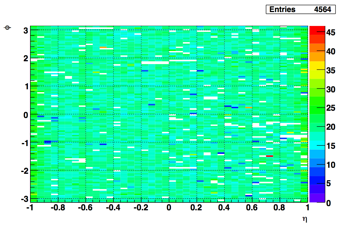
09 MIP peaks calculated using L2W stream
The MIP peaks plotted in the attachment come from the L2W data. 4564 towers had a good MIP peak, 157 towers did not have enough counts in the spectra to fit, and 79 towers had fitting failures. 52 were recovered by hand for inclusion into calibration.
Also attached is a list of the 236 towers with bad or missing peaks.
I compared the 157 empty spectra with towers that did not have good slopes for relative gains calculated by Joe. Of the 157 towers, 52 had good slopes from his calculation. Those are in an attached list.
Fig 1 MIP peak position:
10 Electron E/p from pp500 L2W events
I ran the usual calibration code over the L2W data produced for the W measurement.
To find an enriched electron sample, I applied the following cuts to the tracks, the tower that the track projects to, the 3x3 tower cluster, and the 11 BSMD strips in both planes under the track:
central tower adc - pedestal > 2.5*rms
enter tower = exit tower
track p < 6 and track p > 1.5
dR between track and center of tower < 0.025
track dEdx > 3.4 keV/cm
bsmde or bsmdp adc total > 50 ADC
no other tracks in the 3x3 cluster
highest energy in 3x3 is the central tower
The energies were calculated using ideal gains and relative gains calculated by Joe Seele from tower slopes.
The corrections were calculated for every 2 eta rings and each crate. The corrections for each 2 rings were calculated first and then applied. The analysis was rerun, then the E/p was calculated for each crate.
The calibration constants will be uploaded to a different flavor to be used with the preliminary W analysis.
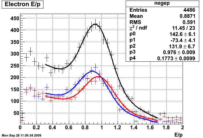
Fig. 1 E/p spectrum for all electrons
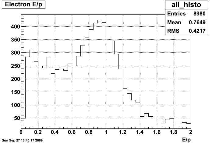
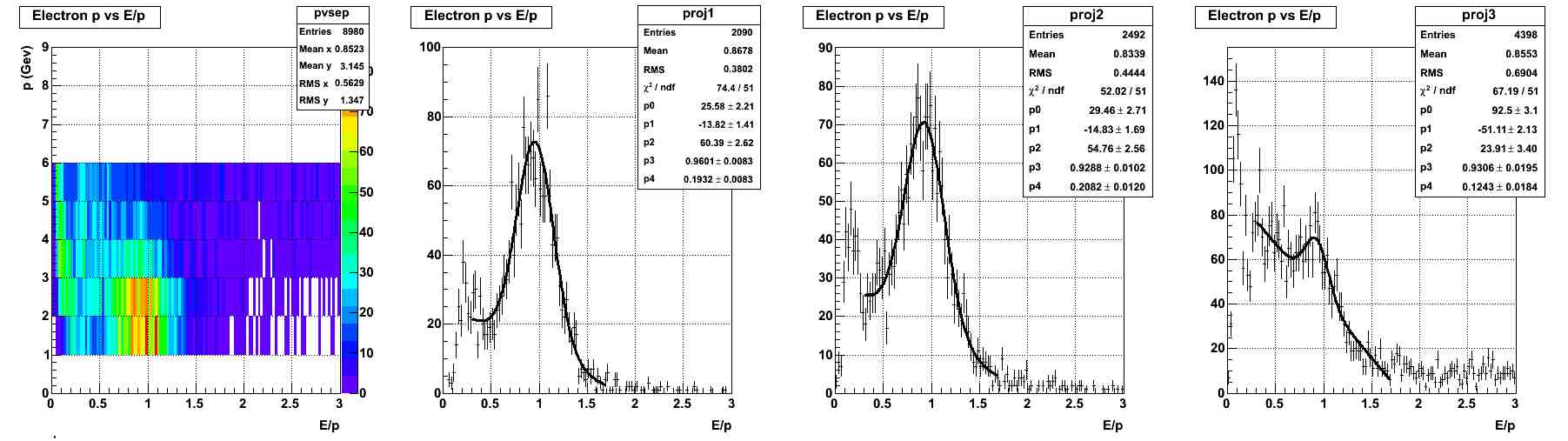
Fig. 2 p vs E/p spectrum for all electrons
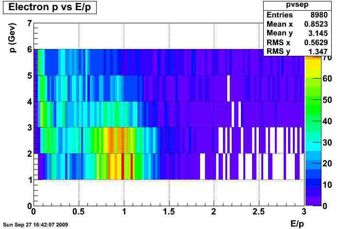
Fig. 3 BSMDP vs BSMDE for all electrons
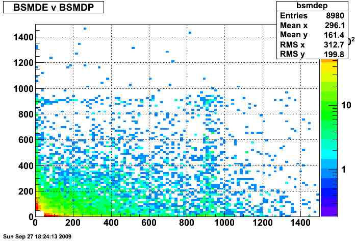
Fig. 4 corrections by eta ring
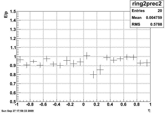
Fig. 5 Crate corrections
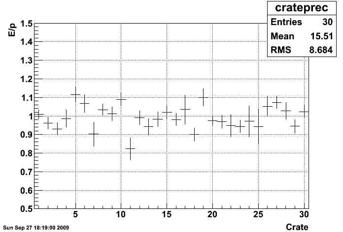
Fig. 6 difference between positrons (blue) and electrons (red):
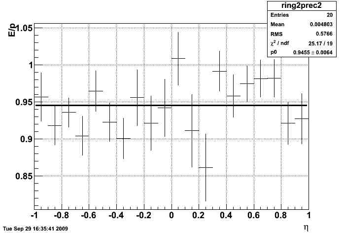
Update: I reran the code but allowed the width of the gaussian to only be in the range 0.17 - 0.175. This region agrees with almost all of the previously found widths within the uncertainties. The goal was to fix a couple fits that misbehaved. The updated corrections as a function of eta are shown below.
Fig. U1
Update 09/30/2009: Added 2 more plots.
Fig. V1 East vs. West (no difference observed)
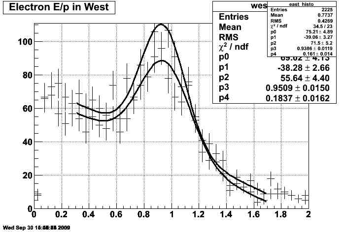
Fig. V2 slices in momentum (not much difference)
Attached are the histograms for each ring and crate.
12 Correcting Relative gains from 500 GeV L2W
After examining the Z invariant mass peak calculated using the L2W data stream with the offline calibration applied, it seemed like there was a problem. The simplest explanation was that the relative gains were reversed, so that hypothesis was tested by examining the Z peak with the data reversed.
The slopes were also recalculated comparing the original histogram to histograms corrected with the relative gains and the inverse of the relative gains.
In the following two figures, black is the original value of the slopes, red has the relative gain applied, and blue has the inverse of the relative gain applied.
Fig 1 Means of slope by eta ring with RMS
.png)
Fig 2 RMS of slope by eta ring
.png)
The E/p calculation improves after making the change to the inverse of the relative slopes because the effect of outliers is reduced instead of amplified.
Fig 3 E/p by eta ring with corrected relative gains
.png)
Update:
After last week's discussion at the EMC meeting, I recalculated all of the slopes and relative gains.
Fig 4 Update Slope RMS calculation
.png)
I then used these relative gains to recalculate the absolute calibration. Jan used the calibration to rerun the Z analysis.
Fig 5 Updated Z analysis
.png)
The updated calibration constants will now supercede the current calibration constatns.
13 Updating Calibration using the latest L2W production
I recalculated the Barrel calibration using the latest L2W production, which relies on the latest TPC calibration. It is suggested that this calibration be used to update the current calibration.
Fit Details:
Negative Peak location: 0.941
Negative Sigma: 0.14
Positive Peak location: 0.933
Positive Sigma: 0.17
<p> = 3.24 GeV
Fig 1. E/p for all electron (black), positive charged (blue), negative charged (red)
.png)
14 200 GeV Calibration
I selected 634 runs for calibration from the Run 9 production, processing over 300M events. The runs are listed in this list, with their field designation.
The MIP peak for each tower was calculated. 4663 towers had MIP peaks found. 38 were marked as bad. 99 were marked as MIPless. The MIP peak fits are here.
The electrons were selected using the following cuts:
- |vertex Z | < 60 cm
- vertex ranking > 0
- track projection enters and exits same tower
- tower status = 1
- 1.5 < track p < 10.0 GeV/c
- tower adc - pedestal > 2.5 * pedestal RMS
- Scaled dR from center < 0.02
- 3.5 < dE/dx < 5.0
- No other tracks in 3x3 cluster
- No energy in cluster > 0.5 central energy
- Track can only point to HT trigger tower if a non-HT trigger fired in the event
Fig. 1: Here is a comparison of all electrons from RFF (blue) and FF (red):
.png)
The RFF fit mean comes to 0.965 +/- 0.001. The FF fit mean comes to 0.957 +/- 0.001. The total fit is 0.957 +/- 0.0004.
Fig. 2 Comparison of electron (red) positron (blue):
.png)
Positron fit results: 0.951 +/- 0.001. Electron fit results: 0.971 +/- 0.001
Calibration was calculated using MIPs for relative calibration and absolute calibration done for eta slices by crate (30 crates, 20 eta slices per crate).
The outer ring on each side was calibrated using the entire ring.
2 towers were marked bad: 2439 2459 due to a peculiar E/p compared to the other in their crate slice. It is suggested this is due to bad bases.
Fig 3 Crate Slice E/p correction to MIPs (eta on x axis, phi on y axis):
.png)
New GEANT correction
A new geant correction was calculated using new simulation studies done by Mike Betancourt. The energy and pseudorapidity dependence of the correction was studied, and the energy dependence is small over the range of the calibration electron energies.
A PDF of the new corrections are here.
Is it statistical?
From this plot, it can be seen that most of the rings have a nonstatistical distribution of E/p values in the slices. The actual E/p values for each ring (for arbitrary slice value) can be seen here.
Comparison to previous years
Fig 4 Eta/phi of (data calibration)/(ideal calibration)
.png)
Fig 5 Eta ring average of (data calibration)/(ideal calibration)
.png)
Issues:
- FF vs RFF (partially examined)
- positive vs negative (partially examinced)
- eta/phi dependence of geant correction, direction in eta/phi
- dR dependence of calibration
- comparison to previous year