jwebb's blog

We use the preshower subsytem to statistically extract single-photon yields in the EEmc. The method is similar to that employed by CDF [1]. An isolated sample of photon candidates is identified above p_T > 5.0 GeV in the endcap. Gamma candidates with charged particles within R < 0.3 are vetoed using the 1st preshower layer. The remaining candidates should be primarily composed of neutral particles. Based on the differential probabilities for 1 versus 2 photons to convert in the first radiator and deposit energy in preshower-2, it is then possible to extract a photon yield.

What follows is a "proof-of-principle" analysis. The biggest "trick" is determining the conversion probabilities for the signal and background events, and this will need to be investigated further to quantify systematic uncertainties.

Contents

0. Extraction of single gamma yields in the EEmc using the conversion method

1. Obtaining an isolated, neutral particle event sample

2. Determining gamma and "background" efficiencies

3. Extracted gamma yields vs pT, eta and "transverse-profile" variables

4. Observations and Conclusions

5. References

0. Extraction of single gamma yields in the EEmc using the conversion method

Method:

First we apply several cuts to obtain an isolated, neutral particle event sample, using the 1st preshower layer as a charged-particle veto (CPV). The cuts will be described below. Then the analysis depends on the measured rate of photon conversions between the 1st and 2nd preshower layers, and the predicted rate of conversions for signal and background. This method has been employed by CDF [1], although their detector was less optimized for it than the endcap preshower subsystem.

Let ε be our measured rate of conversions and N_total the total number of events which pass our isolation and CPV cuts. Then we can write

ε N_total = ε_gamma N_gamma + ε_backgroundN_background (eqn 1)

where ε_gamma is the expected rate of single-gamma conversions and ε_background is the expected rate of background conversions. We can trivially write

N_background = N_total - N_gamma, which allows us to recast equation (1) as

N_gamma = N_total× (ε - ε_background) / (ε_gamma - ε_background). (eqn 2)

If we make the assumption that the backgrounds arise mainly from π⁰ --> 2γ and η --> 2γ decays, then we can calculate the efficiency for the background from the efficiency for a single gamma. The probability that at least one photon converts is twice the probability for a single photon converting, minus a correction for the fact that we have double counted the times when both photons convert--

ε_background = 2 ε_gamma - ε_gamma² (eqn 3)

Our task now is to count the number of photon conversions in the data sample. In order to "count conversions" we will apply the following cut to preshower-2. It casts a wide net on purpose -- if we're dealing with a pi0 decay, we want to have a high probability to catch both photons. Therefore we sum up all preshower-2 tiles w/in R < 0.3 of the photon candidate. An event passes the cut if any one or more tiles shows up with ADC > 3 σ above pedestal.

In the next section we discuss how the cuts are applied. Followin that, we discuss how the efficiencies for signal and background are guess-timated. Finally we look at estimated gamma yields versus pT, eta and quantities which are sensitive to the transverse profile of the shower.

1. Obtaining an isolated, neutral particle event sample

Event sample:

1. Data from ppLong2

2. All fills after L2gamma EEmc elevated to physics

3. List of runs (273)

4. Select trigger ID 137641

Cuts:

We apply the following cuts in order,

1. Require candidate to be w/in the EEMC with pT > 5.0 GeV.

2. Hadronic veto -- require sum of all postshower tiles w/in R < 0.3 to be less that 0.2 MeV energy deposited.

3. Charged particle veto -- require sum of all preshower-1 tiles w/in R < 0.3 to be == 0

4. Isolation cut -- E_T / E_T^R<0.3> 0.9

5. Sum of energy deposited w/in preshower-2 > 0 MeV.

Difference between cuts 4 and 5 is used to extract the gamma yield using equation 2 above --

N_total = Number of events passing cut 4
N_pass = Number of events passing cut 5
ε = N_pass / N_total

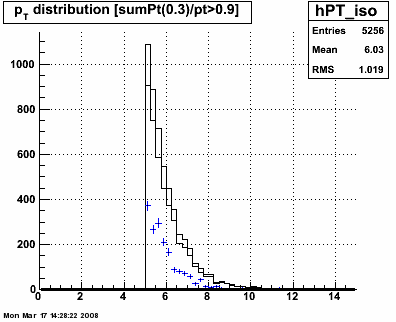
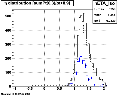
Figure 1.1 -- pT (left) and η (right) distribution for each gamma cut.

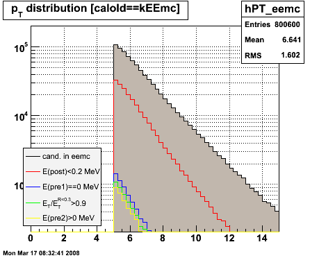
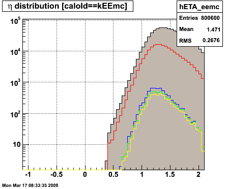
Figure 1.2 -- Isolation distributions for each gamma cut. Isolation sums taken over R < 0.3 (solid lines) and R < 0.5 (dashed lines).

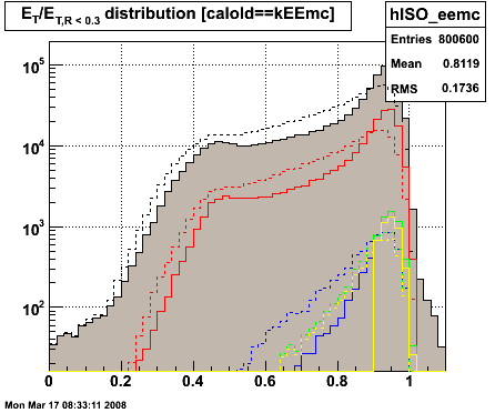
0.2% of events show up with an abnormal isolation sum... more energy within the gamma candidate than when we sum up all towers and tracks w/in R < 0.3. I suspect roundoff differences between the eemc cluster maker and the gamma candidate maker.

Figure 1.3 -- Preshower-1 (left) and preshower-2 (right) response for gamma cuts

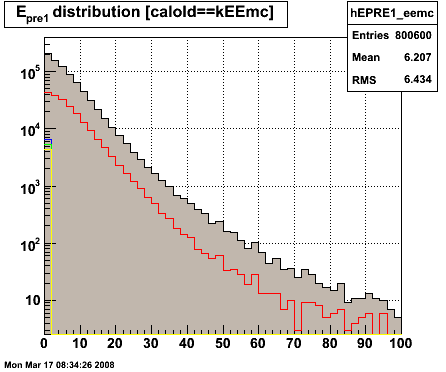
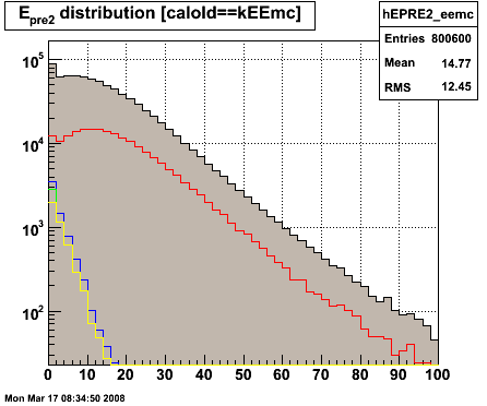
Figure 1.4 -- SMD response for gamma cuts. Energy of SMD strips associated (i.e. +/- 20 strips around gamma centroid) is summed. Divide E_smd by E_tower.

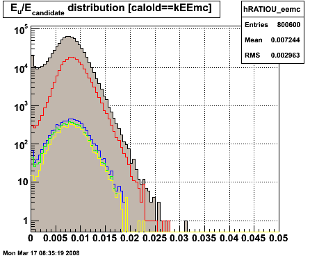
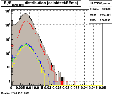
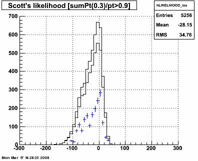
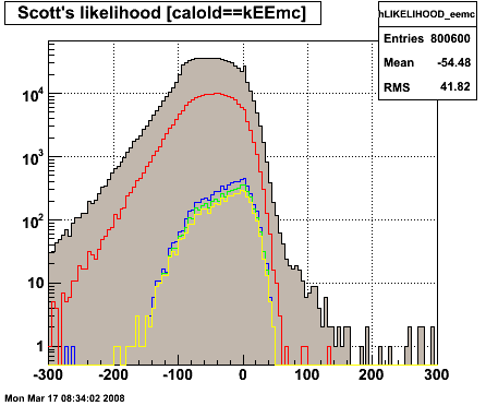
Figure 1.5 -- Likelihood distribution from residual analysis

2. Determining gamma and "background" efficiencies

The trick to extracting yields from the above histograms is to determine the efficiency with which the background and signals will pass the last cut.

The last cut is "energy is deposited in the 2nd preshower layer." We can calculate this in three different ways.

1. Assume that if a photon converts, there will be energy deposited in the 2nd preshower layer. If we neglect epoxy and plastic, there is 0.872 radiation lengths between the 1st and 2nd preshower layers. Conversion will depend upon the angle of incidence. Assuming normal incidence, 50% of gammas convert in the first radiator. Otherwise,

assuming z-vertex = 0 we get

	photon transmission	photon conversion
eta=1.0	41%	59%
eta=1.5	47%	53%
eta=2.0	49%	51%

Assuming that equation 3 above holds and events leave energy in the 2nd preshower detector if they convert, we get ε_π0 = 83.1% to 76.0%, depending on event kinematics.

2. Compare this to a direct measurement using a pi0 sample. After isolation cut I get 102 pions. After applying Epre2 > 0, I get 94. This corresponds to 92 +/- 5% efficiency for a pi0 to convert. This is higher that what we expect based on the amount of material we expect to be in the first radiator. This should be reasonable, our cuts still allow additional neutral particles to be in the vicinity of the pi0's. These additional photons can convert and yield energy in the 2nd preshower layer. A possibility not accounted for in the calculation above.

If we were to assume that the pi0 sample contains only 2 gammas per event, we could estimate (eqn 3) that

ε_gamma = 72.6 +/- 8.0%

3. EEmc Gammas via conversion method, systematics

Throw single gammas and single pi0's at the endcap. Apply all cuts and count:

ε_π0 = 82.3 +/- 1.5%

ε_gamma = 66.0 +/- 1.3%

Conclusion:

The simulated pi0 conversion rate is in line with what we expect from the calculation in "1" above, but inconsitent with the direct measurement in "2". But the simulation neglects the coincident jet. So we use the measured value in "2" of ε_π0 = 92 +/- 5%. The gamma conversion rate measured in the MC is slightly higher than what we would calculate in "1". I suspect this is due to inefficiencies in the charged-particle veto cut allowing some gammas through which showered. We use the result from "3" of

ε_gamma = 66.0 +/- 1.3%.

3. Extracted gamma yields vs pT, eta and "transverse-profile" variables

Figure 3.1 -- Extracted gamma yield vs pT (left) and eta (right). The solid histogram shows events which pass the isolation cut. The dashed lines show the events which pass the preshower-2 cuts. The ratio of those two histograms gives epsilon in equation 2 above. The blue data points show the gamma yields, assuming ε_gamma = 66.0 +/- 1.3% and ε_background = 92 +/- 5%. No systematic errors have been estimated.

Next, look at several quantities sensitive to the transverse shower profile.

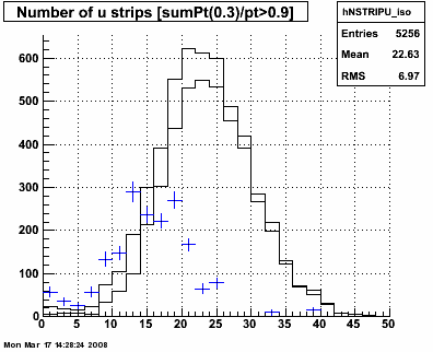
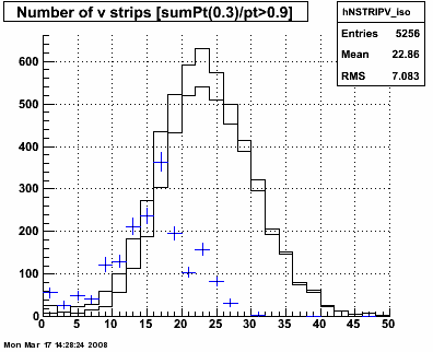
Figure 3.2 -- Number of strips with ADC > 3 sigma + ped w/in +/- 40 strips of gamma centroid. Ngammas are clearly overestimated at small Nstrips. But the qualitative behavior is as we expect -- photons have fewer strips which fired compared with the background.

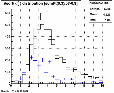
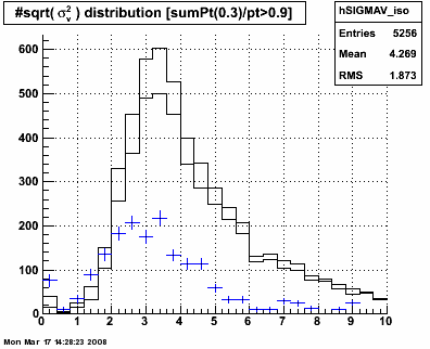
Figure 3.3 -- sigma U and sigma V. Again, the "widths" of the gammas appear qualitatively consistent with epectations. They show up

at smaller sigmas than the "backgrounds". As a consistency check, looking at the distribution of widths extracted from the gamma sample...

Mean sigmaU = 3.36 with an RMS of 1.7. Mean sigmaV = 3.5 with an RMS of 1.7. This can be cross-checked with the "photon library"

which Hal, Will, Pibero et al. are working on.

Figure 3.4 -- The "likelihood" measure developed by Scott and Pibero based on the residual analysis. Things do not look as good as we would expect based on single particle MC.

4.0 Observations and Conclusions

0. Yields are not unreasonable. Between 6-7 GeV, I count approximate 500 gammas based on approximately 2.2 pb^-1 of data (number "chosen" to make the math easy). Compare this to the yields we would estimate for 22 pb-1 using pythia, albeit for gamma-jet coincidences [ref 3, page 13]. There I count about 15k events. Scale up the current estimate by 10 and we would have 5k events. We probably lose 1/2 of our statistics due to conversions in ~1 radiation length of material before the endcap. So this looks even better.

1. The eta-distribution of the extracted gammas falls off above eta = 1.4... if memory serves, this is about where the cross section begins to fall off. (?)

2. There is quite a bit of sensitivity of the yields to the assumptions made for the conversion rates of single photons and "backgrounds". Need to quantify our systematic uncertainties better. Also take into account the known eta-dependence and the suspected pT-dependence of the conversion rates.

3. With these cuts, it looks like we potentially have a ~1:1 signal-to-noise ratio above pT = 6 GeV. (Again, need to refine conversion rates... there are potentially large systematic uncertainties which affect this). This is before any SMD information is included.

4. The transverse shower variables show the qualitative behavior which we expect. Fewer SMD strips hit for gammas than for background. Variance is smaller for gammas than for background. Residual distributions are closer to the "gamma" line than the pi0's in the "likelihood" plots.

5. The gammas show σ_U = 3.35 strips and σ_V = 3.5 strips, which is in nice agreement with what "Will's" selected photons [4] look like.

6. There are clearly some additional clean-up cuts which we can make which would not eat into our yields very much. Specifically: