Run-11 Transverse Jets: dE/dx PID Pion Peaks
It is worthwhile to investigate the behavior of the Gaussian nσ(π) pion peak. If the centroids are close to zero and the widths close to unity, it suggests that the nσ(K) and nσ(p) peaks may be used to set upper limits on the K/p contaminations. This may also allow us to reduce the associated contamination systematic uncertainties.
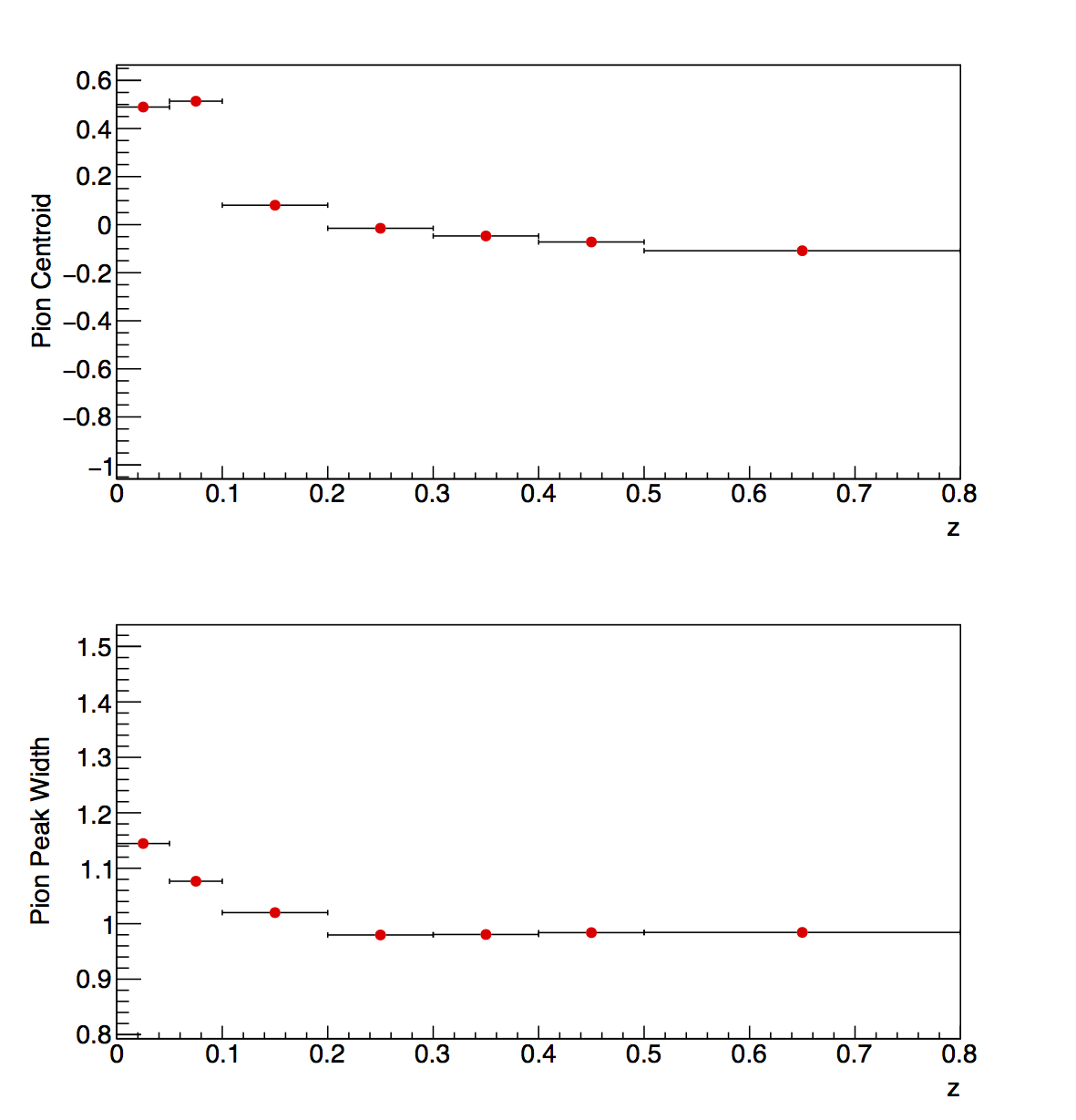
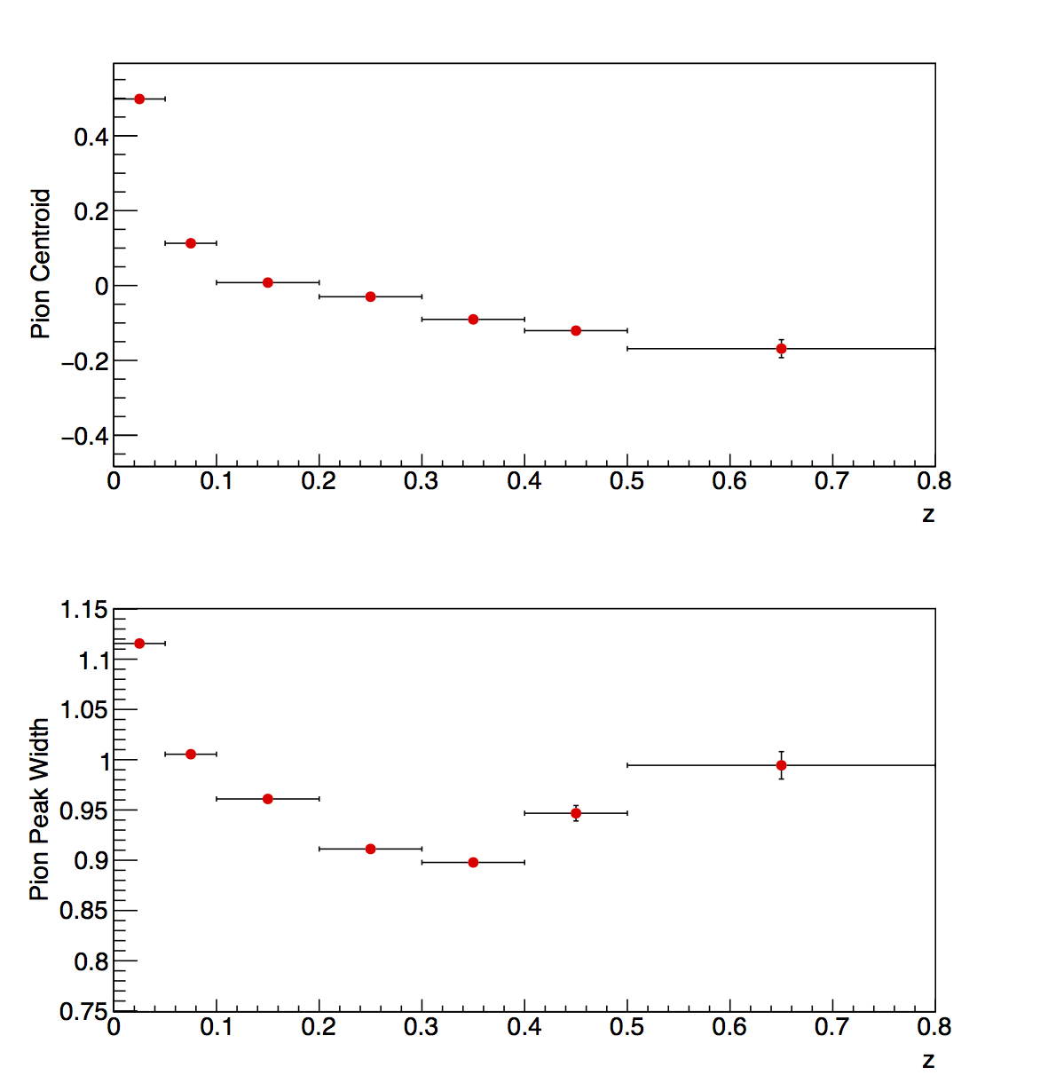
Figure 1: Pion Peaks
| Low pT | Mid pT | High pT |
 |
 |
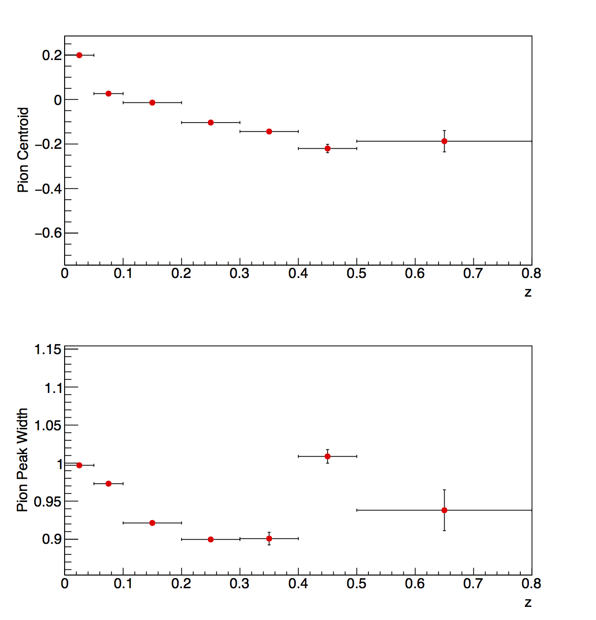 |
Figure 1 shows the results for low, mid, and high-pT as a function of z. The fits are those with the "fixed" electron centroids. Within the relevant window of z, namely 0.1-0.8, The pion centroids range from -0.2 to within 0.1. The widths range from about 0.9 to 1. This suggests the pion peaks behave as proper normal distributions.
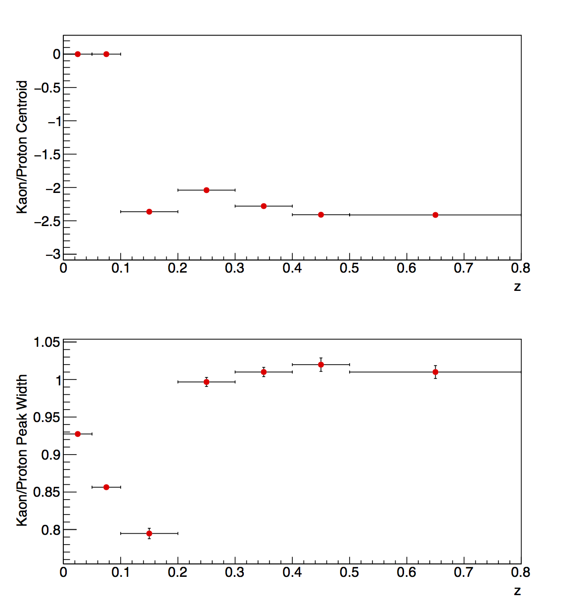
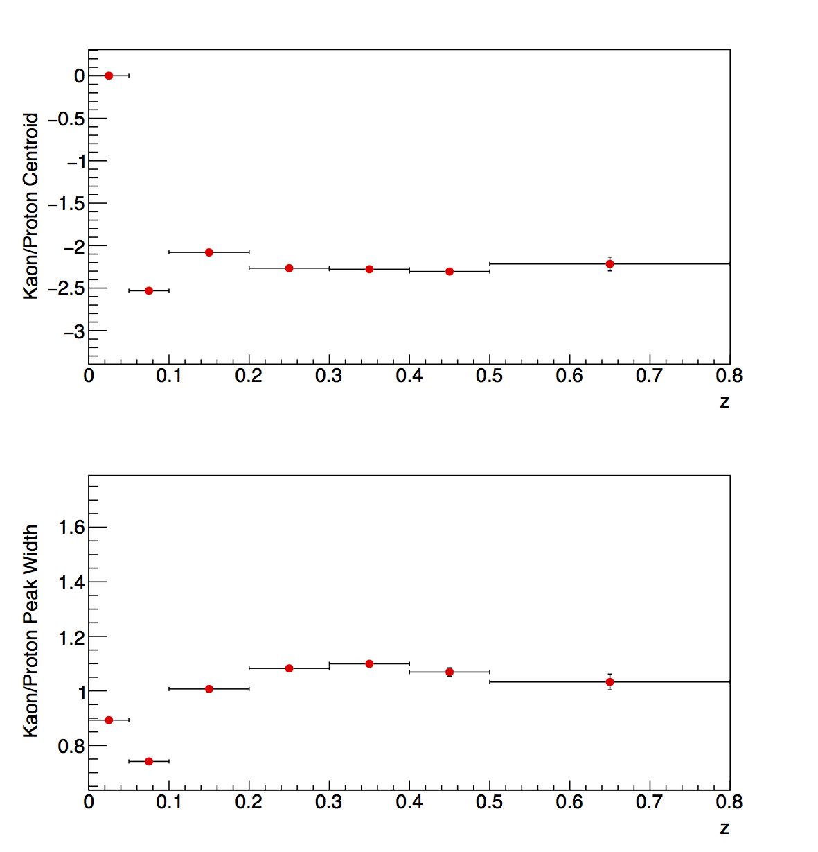
Figure 2: Kaon/Proton Peaks
| Low pT | Mid pT | High pT |
 |
 |
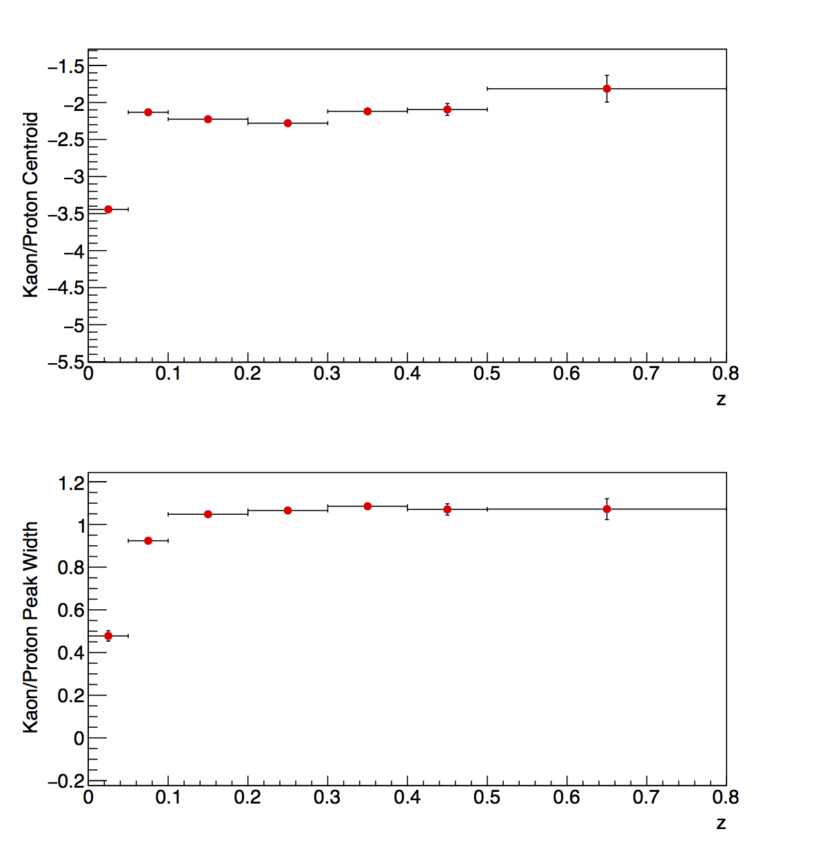 |
Figure 2 presents the centroids and widths of the kaon/proton peaks. Again, the peaks generally behave as proper normal distributions, with widths around 1 and centroids around -2. The 0.1-0.2 bin at low-pT has a bit of a smaller width than one might expect (0.8 vs. 1.0). However, it should be noted that this bin, in particular, has a large kaon/proton contamination that is missed by the dE/dx fits. So, it is perhaps not a surprise if the fit reveals a kaon/proton peak that does not behave as a proper normal distribution. Outside of this bin, in the 0.1-0.8 range relevant for the present measurement, the K/p peaks appear to be normal distributions.
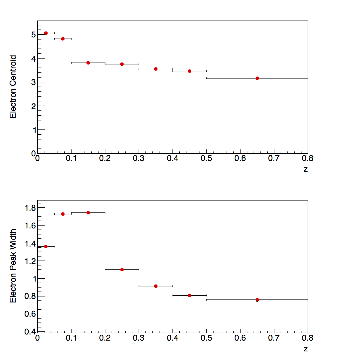
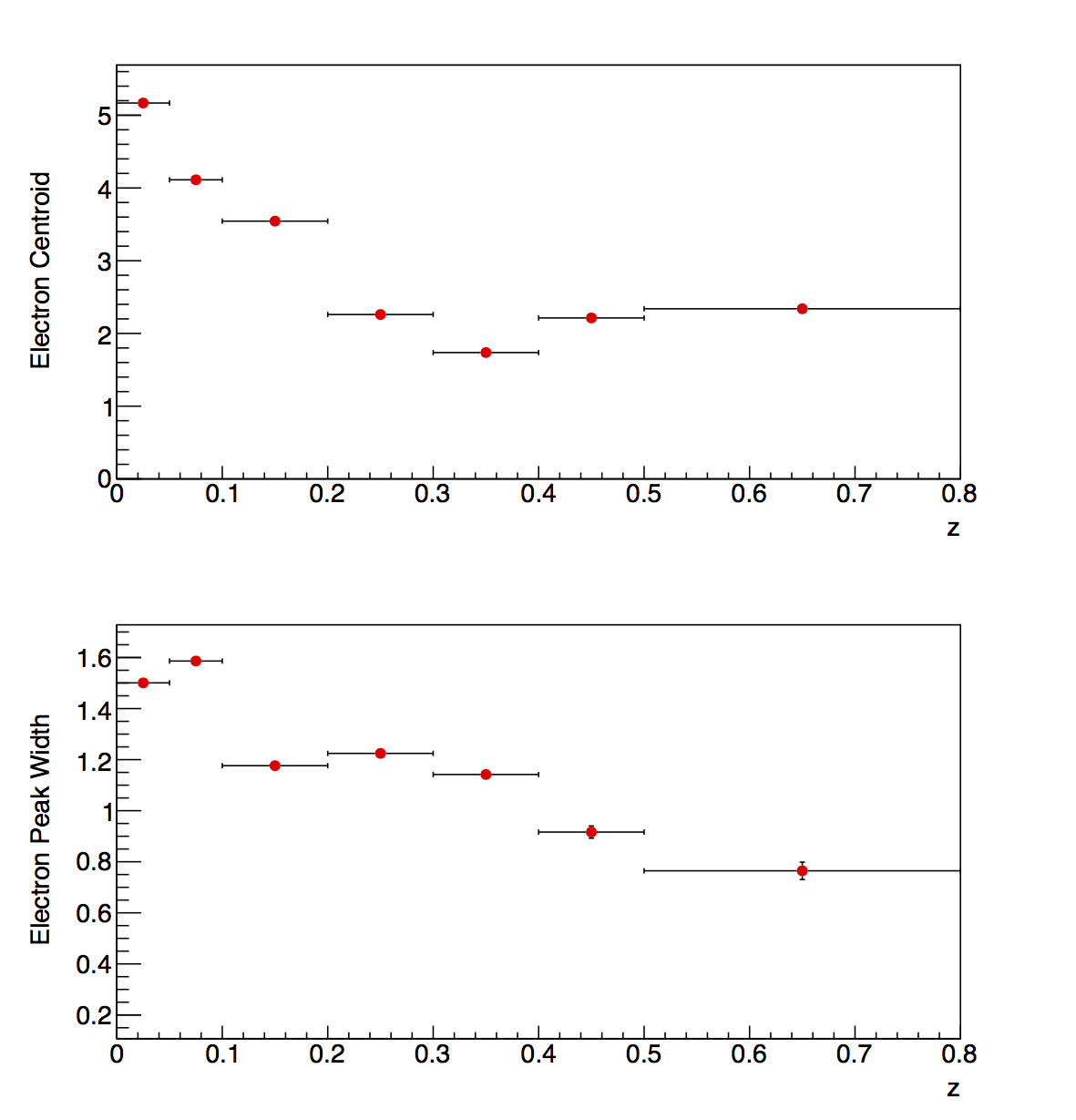
Figure 3: Electron Peaks
| Low pT | Mid pT | High pT |
 |
 |
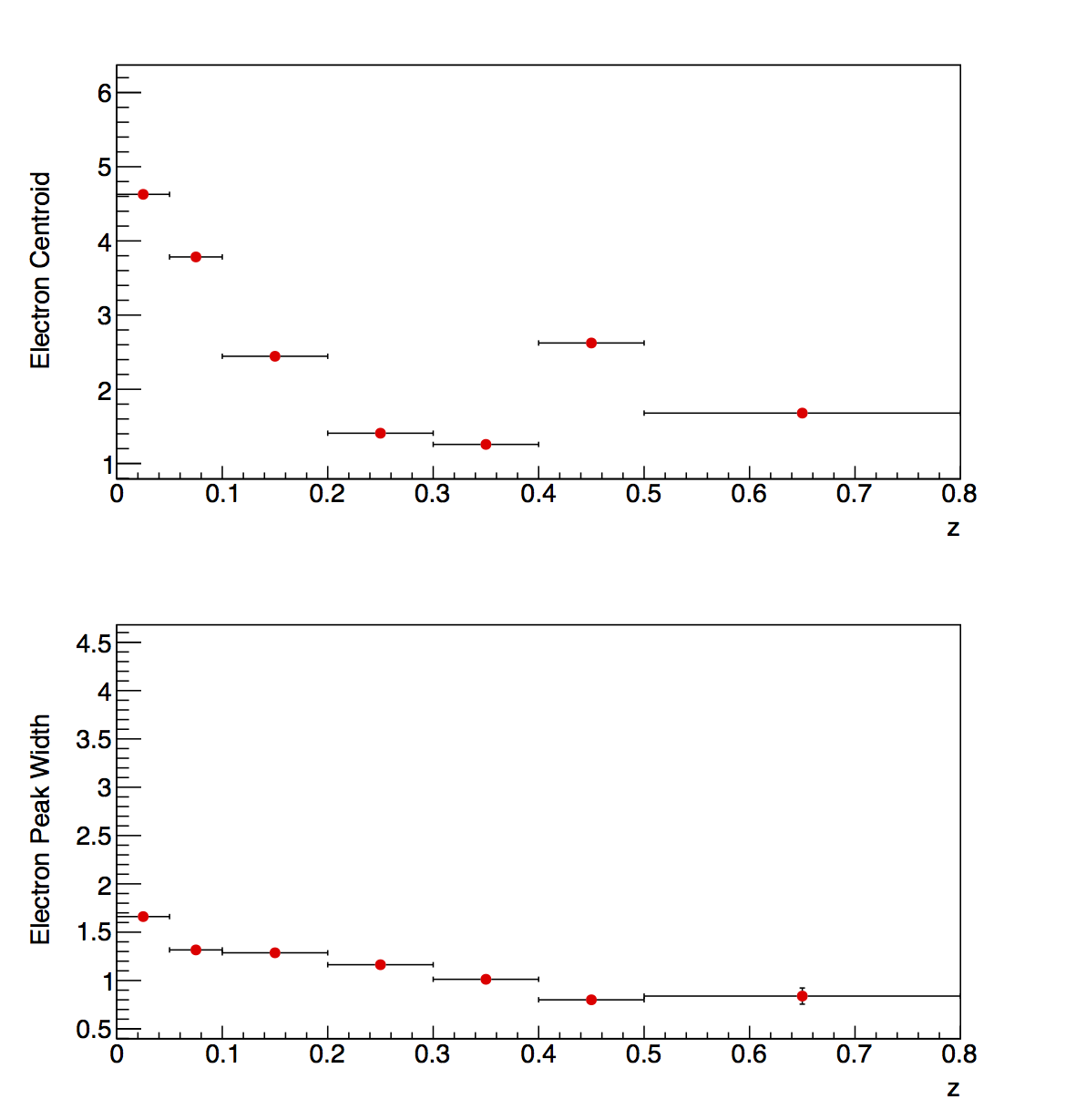 |
Figure 3 presents the electron peak centroids and widths. The electron peaks show a bit more variation than the pion or K/p peaks. Still, within the range of 0.1-0.8, the peak widths are generally within 0.8-1.2. One notable exception is the 0.1-0.2 bin at low-pT. The electron contamination in this bin is found to be rather small, around 1.4%. The larger concern in this bin is the state of the K/p contamination. So, generally, the electron peaks also behave as proper normal distributions.
Having demonstrated well-behaved dE/dx peaks, it should be possible to use the nσ(K) and nσ(p) peaks for setting limits on the contamination above the range where TOF resolution degrades. These distributions were presented on a previous blog entry. The active range is -1 < nσ(π) < 2.5, representing 0.819 of the pion Gaussian. Kaons and protons should manifest as normal distributions, centered at zero in nσ(K) and nσ(p), respectively. The region of the Gaussian nσ(K) and nσ(p) covered can be estimated by marking the horizontal position where the data nσ(K) and nσ(p) distributions "turn on." Arbitrarily, this is estimated by point where the data distribution rises to 18% of the maximum. For conservative (but not crazy) estimates, I assume the kaon and proton yields to be 18% and 12% of the pion yield, respectively, and ignore contributions from electrons.
Table 1: High-pT dE/dx Particle Fractions
| z-Bin | Pion Fraction | K/p Fraction | Electron Fraction | nσ(K) Sampled | nσ(p) Sampled | K Est. (nσ(K)) | p Est. (nσ(p)) |
| 0.1-0.2 | 0.9500 | 0.0321 | 0.0171 | > 1 | > 1.5 | 0.033 | 0.009 |
| 0.2-0.3 | 0.9135 | 0.0416 | 0.0441 | > 0.75 | > 2 | 0.047 | 0.003 |
| 0.3-0.4 | 0.8823 | 0.0629 | 0.0536 | > 0.5 | > 1.5 | 0.063 | 0.009 |
| 0.4-0.5 | 0.9393 | 0.0566 | 0.0034 | > 0.5 | > 1.5 | 0.063 | 0.009 |
| 0.5-0.8 | 0.8822 | 0.0912 | 0.0246 | > 0.25 | > 1.25 | 0.080 | 0.014 |
Table 1 presents the new contamination estimates from the 4-Gaussian fits and nσ(K/p) distributions. The estimates are generally quite close to the total K/p fraction found by the three-Gaussian fits. The two largest deviations are the 0.1-0.2 bin and the 0.4-0.5 bin. For the 0.1-0.2 bin, the fit estimate is 3.2% K/p while the estimate is 4.2% K/p. For the 0.4-0.5 bin, the fit estimate is 5.7% K/p while the estimate is 7.2% K/p.
Table 2: Mid-pT dE/dx Particle Fractions
| z-Bin | Pion Fraction | K/p Fraction | Electron Fraction |
| 0.1-0.2 | 0.9659 | 0.0281 | 0.0056 |
| 0.2-0.3 | 0.9267 | 0.0450 | 0.0278 |
| 0.3-0.4 | 0.8942 | 0.0536 | 0.0512 |
| 0.4-0.5 | 0.9249 | 0.0467 | 0.0271 |
| 0.5-0.8 | 0.9378 | 0.0413 | 0.0191 |
Table 3: Low-pT dE/dx Particle Fractions
| z-Bin | Pion Fraction | K/p Fraction | Electron Fraction |
| 0.1-0.2 | 0.9834 | 0.0012 | 0.0143 |
| 0.2-0.3 | 0.9572 | 0.0399 | 0.0029 |
| 0.3-0.4 | 0.9523 | 0.0448 | 0.0025 |
| 0.4-0.5 | 0.9550 | 0.0424 | 0.0022 |
| 0.5-0.8 | 0.9542 | 0.0414 | 0.0041 |
- drach09's blog
- Login or register to post comments