THE PROBLEM

Some TPC distortions exhibit an approximately linear z dependence in a particular observable. Two notable examples of this are:

1. SpaceCharge distortions increase approximately linearly with z (drift distance) from the endcap. This can be clearly seen in the observable of signed transverse DCAs of tracks which are restricted to have very small pseudorapidity, so-called "straight-up tracks" (i.e. have nearly no slope in z, and are thus reconstructed within a very small slice of z).
2. GridLeak distortions also increase approximately linearly with z (drift distance) from the endcap. An observable in this case is the signed transverse residual of hits on a padrow near the inner-outer sector gaps (i.e. signed residuals along the padrow on padrow 13, or signed residuals on padrow 13 minus the signed residuals on padrow 14).

While these observables have proven powerful in measuring these distortions and correcting for them, pile-up contributions to the observable can affect the z dependence, because pile-up is randomly distributed in reconstructed z. Over the years, I have tried to reduce pile-up contributions through certain cuts, like using only global tracks which have a primary partner associated with the highest ranked vertex, and only for vertices with at least some minimum number of daughter tracks. But pile-up You do not have access to view this node.

With the pp500 data acquired during Run 9, pile-up reached new highs in conjunction with the highest luminosities ever seen by the STAR TPC.

ILLUSTRATION OF THE PROBLEM AND SOLUTION

Joe Seele and I thought about this and came up with a scheme to deal with it, as the following plots hopefully demonstrate. The plots show a distortion observable (e.g. either of the two above-mentioned ones) versus reconstructed z, or more accurately a profile (or average) of some observable versus z. The red line denotes the observable from triggered events, which are reconstructed at the true z and what we hope to properly correct. The blue line denotes how pile-up contributions to the observable are reconstructed (not necessarily at their true z), and the black line represents the weighted average of the blue and red, where the weighting comes from the amount of pile-up which leaks through the cuts (i.e. higher luminosities will make the pile-up to triggered ratio larger and move the black line closer to the blue line).

In the uncorrected case, triggered events show a z dependence which starts at zero near the endcap (zero drift length), linearly increasing towards the central membrane. Pile-up is randomly reconstructed in z, so it shows a z dependence which is flat, and a magnitude representing the average of all collisions over all z.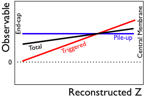
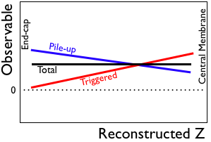
Once you've applied any correction at all, the slope as a function of z changes for both the trigger data and pile-up data. Therefore, reducing the total slope to zero is NOT the thing to do, as all it means is that the distortion corrections are performing a balancing act between pile-up and trigger data. It implies that such a distortion correction is too small. [N.B. Wrong as it may be, this is the method which has been practiced in recent years, including the Run 9 pp200 calibration.]
Even making the total distortion go to zero at the central membrane is still too small.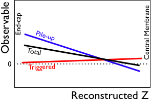
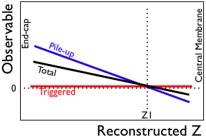
However, there is a point in z (Z1) on each half of the TPC where the observable is the same for pile-up and triggered data. Finding Z1, and bringing the observable to zero at Z1 is what we want. Importantly, please note that this point is independent of the weighting of pile-up contributions versus the triggered contribution to the observable!

FINDING Z1

Z1 represents the point at which the average of the observable over all z and all collisions is equal to the value of the observable at that z for triggered collisions. If I use D(z) to represent the distortion observable as a function of z, and g(z) to represent the distribution in z of the contributors (e.g. tracks) from triggered collisions, then I may state this mathematically as:

  D(Z1) = ∫dz { D(z) g(z) } / ∫dz { g(z) }

where the integral is over z from the central membrane to the endcap. One may prefer to use a normalized version of g'(z), where the integral over z is 1, and

  D(Z1) = ∫dz { D(z) g'(z) }

[N.B. Before going too far, one should recognize that the left and right sides of this equation are different in a major way: the left side may be a single value for a specific location in z, while the right side represents an average of values. In practice, this means that the right side may appear as a diffuse distribution of the observed value at a given z, whose average is equal to the single value from the left side of the equation. Reality is even less well-defined, because even the observable for triggered events may have dependencies on things like which padrows are included in a track fit, and so may be seen as a distribution for a given z. So I should reiterate that we are in the end looking at profiles (averages) of these observables as a function of z.]

So Z1 is dependent on the distribution function, which itself is dependent on the observable being used. Furthermore, as noted earlier, D(z) for the cases in which we are interested is approximately linear in z and may be approximately written as

  D(z) = C₀ (205-|z|)

where 205 represents the point (close to the endcap) where the distortion observable goes to zero (z=0 is the central membrane). Don't forget that there's a Z1 on each half of the TPC, but if we assume symmetry across z=0, then we may restrict ourselves to positive z (though the plots above were drawn for negative z...sorry). In that assumption, we may write:

  Z1 = 205 - ∫dz { (205-z) g'(z) }

CASE 1: GRIDLEAK

Tracks used for observing the GridLeak distortion via residuals near the inner-outer sector gap come from all z. Fortunately, if we assume a flat pseudorapidity dependence (as is approximately true over the +/-1 units of pseudorapidity which STAR covers, and to which we may restrict ourselves in this calibration [or even tighter if we choose]), then the z distribution of contributions to the residual measurements should be essentially flat as a function of z regardless of the z distribution of collisions generating those tracks (i.e. the z distribution of tracks crossing a given radius is independent of z). This makes the integrals rather simple:

  g_GL(z) = C₁
  g'_GL(z) = 1/205
  Z1_GL = 205/2 = 102.5 cm

CASE 2: SPACECHARGE

If we are restricting ourselves to straight-up tracks, then the true z distribution of contributions to the signed DCAs will be equivalent to the true distribution of primary collision vertices. If that distribution can be found accurately, one could use a histogram of the distribution and calculate the integrals numerically, or via Monte Carlo for any functional form (Joe has implemented a tool for the latter). Assuming a Gaussian shape, the integrals can be done analytically:

  g_SC(z) = C₂ exp{-0.5 (z-μ)²/σ²}

Assuming a Gaussian centered at zero makes things a bit easier, but this could be done for a distribution which is not centered at zero (note that such a distribution will have different Z1 values for the two halves of the TPC!). As long as 3σ<205, plugging in μ=0 leads to a final result of:

  Z1_SC = σ√(2/π)

There is the matter of GridLeak contributing to the signed DCA as well. However, if we are restricting to straight-up tracks when looking at signed DCAs, then the distortion function as a function of z changes only by a scale factor, which drops out of the formulas anyhow.

  D(z) = C_SC (205-|z|) + C_GL (205-|z|) ≡ C₀ (205-|z|)

There may also be open questions about how well we know the true collision vertex distribution given cuts placed at the trigger level on collisions being within some window about the center of STAR. There is certainly some tolerance for error in understanding this distribution, but it would require additional study beyond what is presented here. Joe's Monte Carlo tool may be ideal for such a study.

CONCLUSION

The simple result then is to find the SpaceCharge and GridLeak distortion corrections which result in signed DCAs which are 0 at the points z = ±σ√(2/π) where σ is the Gaussian width of the true primary vertex distribution, and residuals on padrows 13 & 14 which are 0 at the points z = ±102.5 cm. This could be improved to take into account other, more accurate primary vertex distributions.

The same methodology may be useful for other z-dependent TPC distortions.

Note that the restriction of using straight-up tracks cuts severely into the statistics of good tracks. The Event-by-Event SpaceCharge correction method in particular would likely be handicapped to the point of no longer functioning. So further developments which could relax this restriction would be valuable.

-Gene