This is the result of work I am doing with Amal Sarkar, and is an update of my Initial look at cosmic ray resolutions.

 

STUDY OF TPC MOMENTUM RESOLUTIONS USING COSMIC RAYS

 

TOC:

Expectations
Using Cosmic Rays
I. Versus p_T
II. Versus Z
III. Versus Sector
IV. Versus Length and Number of Points
V. Influences From Modified Length
VI. Same Sector Restriction
VII. Similar Length Restriction

 

Expectations

In the TPC Chapter (4) of the STAR CDR (see SN0499 : STAR Conceptual design report), equation 4C-14 on page 4C-19 reads (essentially) as follows:

(δp_T/p_T)² = (p_T² σ_φ² 720)/[e² B² s⁴ (n+6)]  +  (3 x 10^-3)/(B² s L_R β²)

where e is a constant (0.2998), B is the magnetic field, s is the track length, n is the number of position measurements (hits), L_R is the radiation length of the drift gas, β is the particle velocity, and σ_φ is essentially the hit position resolution along the padrow. The second term is the multiple scattering contribution, which becomes negligible at high p_T. The use of (n+6) probably relates to the six parameters of a helix, which is perhaps not strictly correct for a Kalman track, but I will continue to use it for now. SN0014 : E and B Field Precision Constraints from Momentum Resolution Requirements in the STAR TPC is referenced for this formula in the CDR, but I have obtained a copy of it and provides no further explanation of from where the numbers 720 and 6 come. Maybe someone else knows.

Further, using δ(1/p_T) = δp_T/p_T²  (assumes small δp_T), we find:

δ(1/p_T) = √{  (σ_φ² 720)/[e² B² s⁴ (n+6)]  +  (3 x 10^-3)/(p_T² B² s L_R β²)  }

Although different tracks will have hits on different padrows, and inner padrows will have a different σ_φ from outer padrows, I will for now ignore this and write that at high p_T the dependence goes like:

δ(1/p_T) = W / [s² √(n+6)]

where W is a constant. Thus the resolution is expected to be constant at high p_T, other than dependences on 1/s² and, approximately, 1/√n. At all p_T, one can use:

(1/β²) = (1 + m²/p²) = (1 + m² cos²θ/p_T²)

where θ is the dip angle and m is the particle mass (so m² ≅ 0.01 for muons), to get a more complete form:

δ(1/p_T) = √{  U/[s⁴ (n+6)]  +  [V (1 + m² cos²θ/p_T²)]/(s p_T²)  }

where U = W². In all sections below (except the ones of p_T dependence), I will place a cut on momenta above 1 GeV/c to try to stay within the simpler high p_T parameterization.

 

Using Cosmic Rays

Steps:

1. Run BFC on daq files.
2. Loop over MuDsts to create an ntuple with track pairs (some events have more than 2 tracks, and all combinations are tried), labeling the track with the higher y value (vertical position) of its last hit as track "1", and so assuming it is the incoming track.
3. Loop over ntuple to find pairs where tracks are back-to-back in polar and azimuthal angles.
4. Plot (q₁/p_T1)-(q₂/p_T2) versus various quantities.
5. FitSlicesY using a Gaussian and then plot the means Δ(1/p_T), and widths divided by √2 to represent single track resolution δ(1/p_T).

These steps are encapsulated in the two macros attached to this page: ProcCosmic.C and ResoCosmic.C

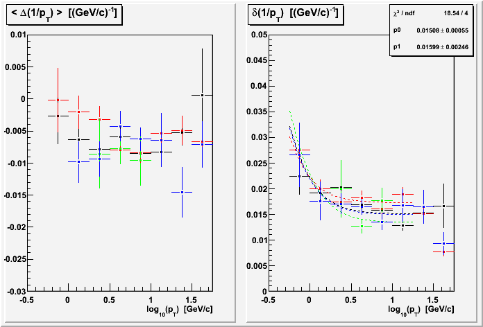
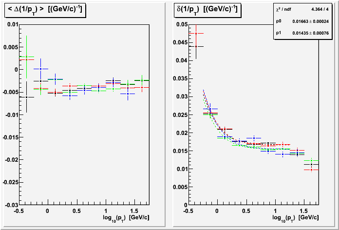
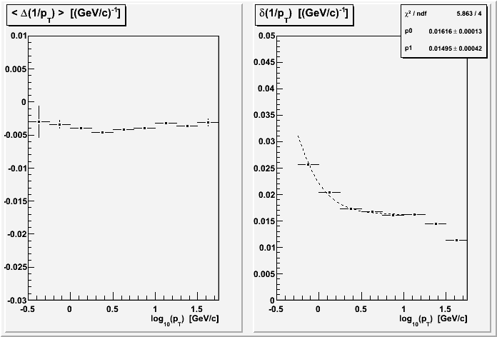
The plot pairs below are the above-mentioned means (left panels) and single track resolutions (right panels) for a portion of the cosmic ray data acquired on June 8, 2010 (day 159) with different anode voltage settings, intended to help understand what impact on momentum resolution to expect from reduced anode voltages if we decide to run that way in the future. There are two groups of triggers: those using the MTD in coincidence with a TOF pair (left plot pairs), and those not using the MTD but just a TOF pair (labeled the "TOF group", right plot pairs).

As a side note, I also learned that I couldn't use events with more than a handful of tracks because some of them appear to be a few Au + X collisions near STAR (tests were ongoing in the collider to see if Au beams could be accelerated to deliver 5 GeV collisions). This I will document on a Cosmic ray events with high multiplicity.

 

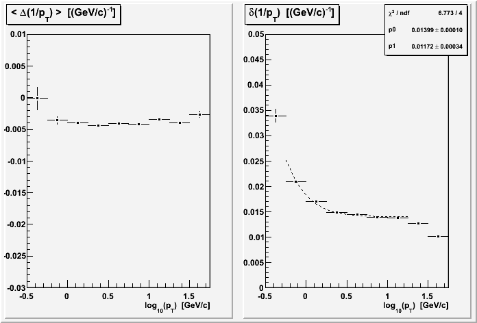
I. Versus p_T

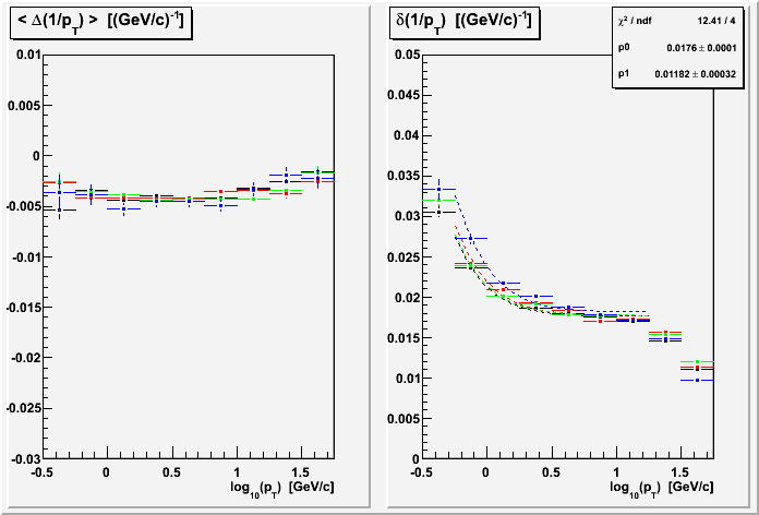
The results here show systematically over different voltage runs two important things:

1. Resolutions are not flat vs. p_T at high p_T (they seem to improve above ~20 GeV/c; this remains to be understood).
2. Resolutions appear to have no significant dependence on anode voltage in the range of voltages tested.

The different colors show different anode voltage settings:

• Black : run 11159020 : 1135V / 1390V (inner / outer)
• Red   : run 11159008 : 1100V / 1390V
• Green : run 11159010 : 1100V / 1345V
• Blue  : run 11159015 : 1070V / 1345V

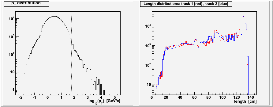
The horizontal axis is actually log₁₀(p_T), so the plot extends from 1 GeV/c to 50 GeV/c, where p_T ≡ 2/((q₁/p_T1)+(q₂/p_T2)), since we really measure curvature and determine p_T from its reciprocal (I am in essence taking the average measured charge-signed curvature). Here the fit ignores track length, dip angle, and number of hit dependencies and is as follows: δ(1/p_T) = √{ p0²  + p1² (p_T^-2 + 0.011 p_T^-4) } :

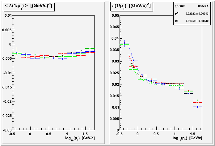
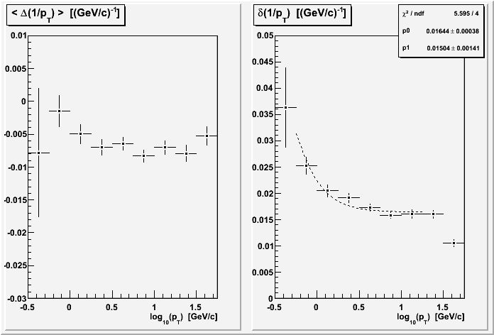
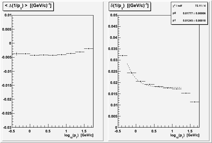
Combining all the voltage sets (for most of the rest of the plots on this page), I get these results for MTD and TOF triggers:

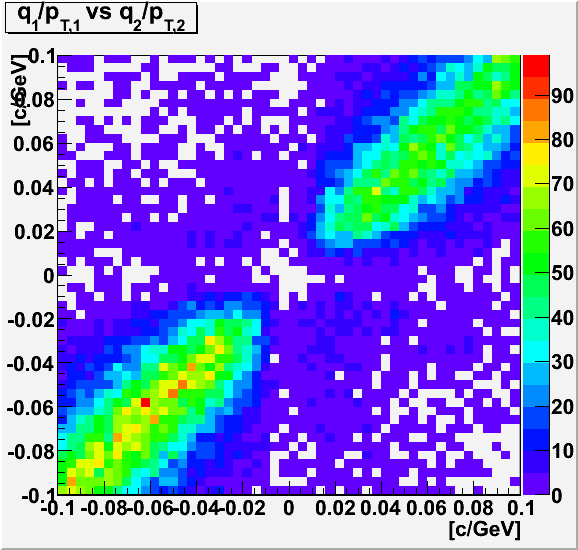
One thought I had was that at high p_T the determination of charge sign for the tracks as a pair could be affecting the determination of pT. But the left (first) plot below of q₁/p_T1 vs. q₂/p_T2 (for the TOF group) shows that there is a pretty clear non-ambiguity of charge sign, which is made from the position of the point either below-left or above-right of the diagonal line from top-left to bottom-right.

The second plot below shows the reconstructed cosmic ray p_T distribution along with dashed lines marking the range used in the above plots of [-0.5,1.75] GeV/c, where the bulk of statistics are. Above and below this range the distribution shape changes and is perhaps dominated by the momentum resolution rather than the true distribution of momenta. Note that the y scale is logarithmic.

I include a third plot showing the distribution of lengths for tracks 1 [red] and 2 [blue]. The y scale is logarithmic, so the distribution is truly dominated by full length tracks. Some additional bumps appear at intermediate lengths due to discrete dead TPC sections (e.g. RDOs).

 

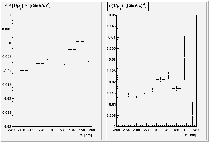
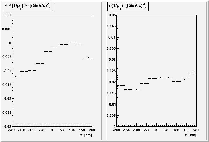
II. Versus Z

Here I calculate z as the average of the z positions of the four points corresponding to the first and last points on the two global tracks.

There seems to be a significant Δ(1/p_T) offset between the first and second track for east side sectors (z < 0), which isn't there for west side sectors (z > 0). There should be some energy loss, which would result in a negative value on this plot, but I'm not sure how much. So it isn't obvious to me at first glance whether the west side shows too little energy loss, or the east side too much. We need to do some math.

The resolutions seem to get worse near the central membrane and endcaps.

 

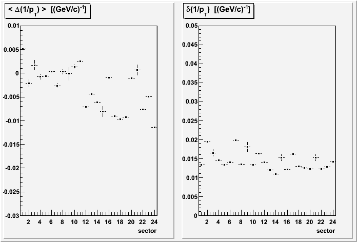
III. Versus Sector

First and last points on tracks are required to stay within a sector. In these plots, I have combined data for the first and second tracks as these are generally non-overlapping groups of sectors. Sectors 3,9,15,21 seem to suffer from being horizontal.

The TOF group shows that there are a few other sectors with notably bad resolutions: 2 and 7 are really bad, while 8,11,17 are also worse than average.

Also making an appearance is the east-west offset in Δ(1/p_T) noted earlier in the z dependence (sectors 1-12 are on the west, 13-24 on the east).

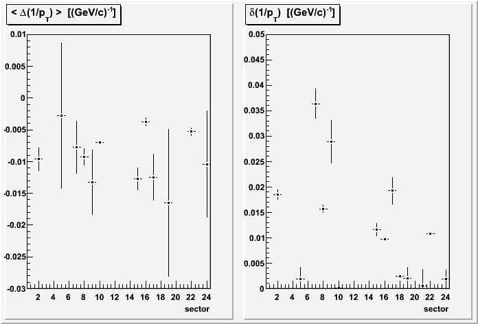
It should be kept in mind that each sector's resolution is determined while using a second track from another sector. This means that if the sector just opposite the one in question has a poor momentum resolution, it could affect the observed resolution for the sector in question.

 

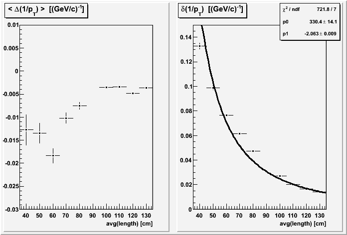
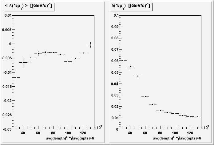
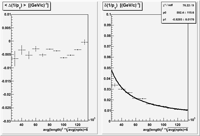
IV. Versus Length and Number of Points

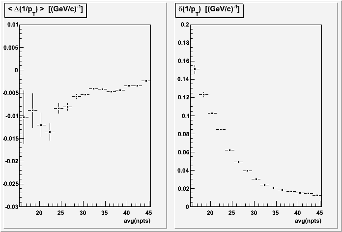
As noted in the Expectations section earlier, the high pT regime should show a s^-2 dependence on track length. Here I calculate the length as the 2D radial distance between the first and last hit points on tracks. I then take the average of the two track lengths to get a single average length. This is shown on the left for the full TOF group of triggers. I similarly calculate the average number of hits on the tracks, shown on the right, expected to depend as approximately n^-0.5.

The data does appear to show a s^-2.06 dependence, but the number of points dependence is actually somewhat similar to the length dependence:

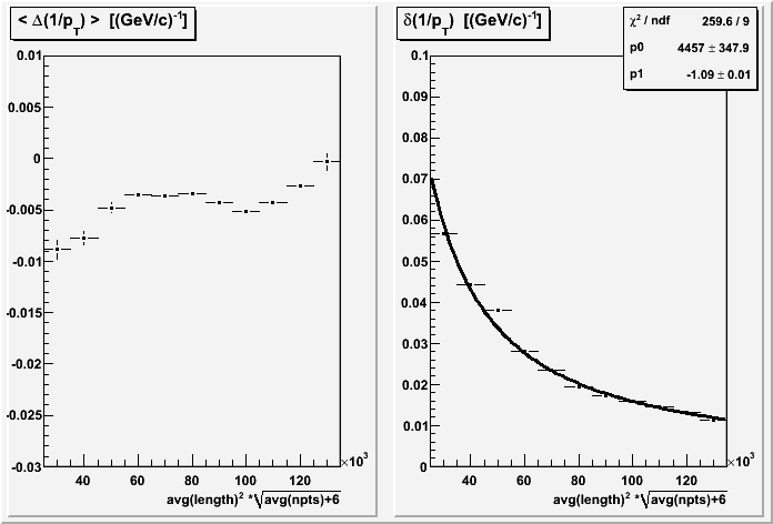
The reason is a (to be expected) correlation between the number of hits and the track lengths. One option is to fit to the expected dependence of a modified length M = s²(n+6)^0.5 and hope for a M^-1 dependence. What we see is M^-1.09, which isn't too bad:

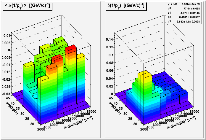
I can take this a step further and fit the s and n dependencies separately. Here I use s² as one axis, in order to better distribute the statistics among the bins, and the fit is to the function p0*pow(s²,p1)*pow(n+p3,p2), where parameter p3 would be 6 in the expected formula, and I've constrained it to be in [0,10] in my fit. Unfortunately, the fit is rather poor, with the parameters not quite as close to expected as one might like to see (and parameter p3 bumps against its boundary at zero):

It may be possible to get better results by constraining the lengths for tracks 1 and 2 to be similar, such that intermediate average lengths are not found through combinations of one short (worse resolution) and one long (better resolution) tracks, since the dependence on length is non-linear. This is investigated below in Section VII.

 

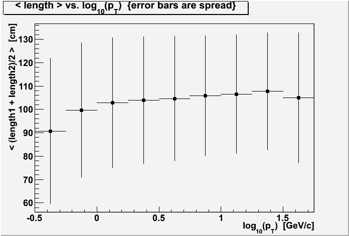
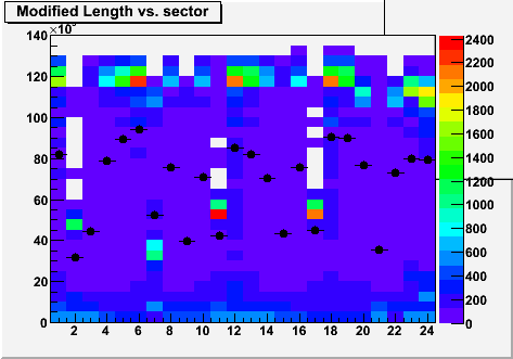
V. Influences From Modified Length

As there is a clear and strong dependence of resolution on either length s or modified length M = s²(n+6)^0.5, δ(1/p_T) ~ s^-2, δ(1/p_T) ~ M^-1, it is important to ask whether any of the previous observations may have been influenced by biases on s or M. Here are two relevant plots using the TOF group of data.

The first plot is the mean avg(length) vs. log₁₀(p_T), with error bars representing the distributions' spreads (not the errors-on-the-mean, which are smaller than the markers). It shows that there is no significant increase in length for high p_T cosmics, thereby ruling out that the downturn seen at high p_T in Section I is due to track length evolution with p_T.

The second plot is M vs. sector, where M was calculated for sectors of track 1, and then for sectors of track 2, and the two histograms then combined. The colored bins show the distribution, while the black points show profile means. It is obvious that several sectors have predominantly small modified lengths likely due to dead regions (2,7,11,17). Some additional sectors have low means perhaps because they are horizontal and the trigger is inefficient there (3,9,15,21). There are a few others which are mildly low. I'm a bit surprised to see that sector 20 is among the latter, and not more significantly affected by its dead region in anode channel 20-5. These lists do match pretty well with the observations in Section III on sector dependence, with perhaps the exception of sector 8 looking on the worse end of the distribution there, but rather middle-of-the-pack here.

The conclusion is that if one really wants to compare resolution performance between sectors neglecting the effects of dead regions, the modified length dependence must first be accounted.

 

VI. Same Sector Restriction

Some tracks cross sector boundaries, so their first and last points are in different sectors. Restricting tracks to stay within a sector (which was already done in Section III on sector dependence) is expected to improve resolution as missing hits across the sector boundaries should degrade resolutions. Here are plots for the TOF group of data for the log₁₀(p_T) (separated by run, and then all combined together), z, and modified length dependencies.

The overall resolution definitely improves, dropping closer to 1.6% at intermediate p_T (compared to ~2.0% in Section I).The structure seen in the z dependence in Section II remains. However, the dependence on modified length appears to be significantly changed (improved?) at small modified length. I have not tried to assess why.

 

VII. Similar Length Restriction

Because of non-linear dependence on modified length, it is worthwhile to see the effects of placing a restriction on modified length (Jamie reemphasized this point). With the inverse dependence, I chose to restrict to |Δ(1/M)| = |(1/M₁ - 1/M₂| < 2e-5. The effects are significant. Here are the TOF group separated and combined results vs. p_T:

Combining the same sector and similar length restrictions gives the best resolution results yet of 1.4% in the intermediate p_T plateau:

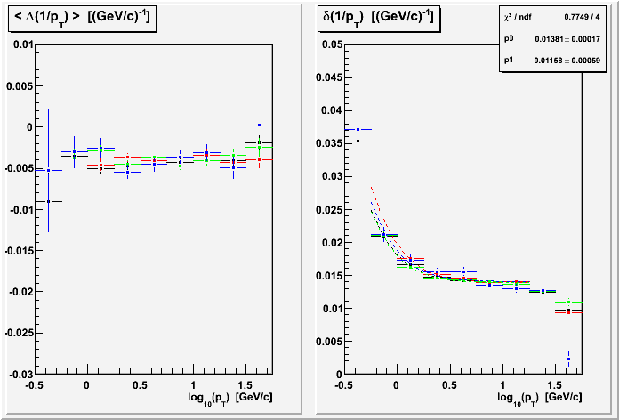
Without further understanding of the still-present drop-off at high p_T (i.e. an unknown systematic), I am myself hesitant about making any statements on the true significance of differences between the fits for different anode voltages (the different runs).

The similar length restriction does make for less dispersion among the sectors, shown below, thought the same sectors still stand out: 2,7,11,17 in one class, and 3,9,15,21 with larger error bars (the horizontally situated sectors) in another.

Taking yet another look at the modified length dependence with these two restrictions in place gives a fit result of M^-0.93:

 

_______________________________

-Gene