- genevb's home page
- Posts
- 2025
- 2024
- 2023
- 2022
- September (1)
- 2021
- 2020
- 2019
- December (1)
- October (4)
- September (2)
- August (6)
- July (1)
- June (2)
- May (4)
- April (2)
- March (3)
- February (3)
- 2018
- 2017
- December (1)
- October (3)
- September (1)
- August (1)
- July (2)
- June (2)
- April (2)
- March (2)
- February (1)
- 2016
- November (2)
- September (1)
- August (2)
- July (1)
- June (2)
- May (2)
- April (1)
- March (5)
- February (2)
- January (1)
- 2015
- December (1)
- October (1)
- September (2)
- June (1)
- May (2)
- April (2)
- March (3)
- February (1)
- January (3)
- 2014
- December (2)
- October (2)
- September (2)
- August (3)
- July (2)
- June (2)
- May (2)
- April (9)
- March (2)
- February (2)
- January (1)
- 2013
- December (5)
- October (3)
- September (3)
- August (1)
- July (1)
- May (4)
- April (4)
- March (7)
- February (1)
- January (2)
- 2012
- December (2)
- November (6)
- October (2)
- September (3)
- August (7)
- July (2)
- June (1)
- May (3)
- April (1)
- March (2)
- February (1)
- 2011
- November (1)
- October (1)
- September (4)
- August (2)
- July (4)
- June (3)
- May (4)
- April (9)
- March (5)
- February (6)
- January (3)
- 2010
- December (3)
- November (6)
- October (3)
- September (1)
- August (5)
- July (1)
- June (4)
- May (1)
- April (2)
- March (2)
- February (4)
- January (2)
- 2009
- November (1)
- October (2)
- September (6)
- August (4)
- July (4)
- June (3)
- May (5)
- April (5)
- March (3)
- February (1)
- 2008
- 2005
- October (1)
- My blog
- Post new blog entry
- All blogs
HFT material accounting in Sti for Run 14 AuAu15 preview production
HFT material accounting in Sti for Run 14 AuAu15 preview production
This is specifically for the state of the HFT materials as they were in SL14d for the April 2014 preview production. We will likely modify and improve upon these representations of the HFT geometry.
_______
Materials are added separately for PXL, IST, and SSD.
Observations of note:
Plots:
As a metric of the effect on track projections with the accounting of material, I used <|ΔDCA|> for global tracks which had at least 25 TPC hits, 0.3 < pT < 2.0 GeV/c, and the 2D DCA to the BeamLine was within 2 cm (i.e. the track did not need to be close to a primary vertex, though the "beamline" was defined by the highest ranked primary vertex (x,y)). For the plots which use non-zero radius, I only made a correction to the z location via z + radius * (η/0.88), which is reasonable to first order for the precision of the plots I have made (the radii I used are only meant to be rough approximations for where material might be anyhow). Some additional explanations follow in the outline of what is presented:
There are a lot of plots, so please read the explanations first...
(Note: images may be opened in another browser window/tab for higher resolution, or clicked on for PDF versions. All distance units are [cm])
_______________
Let's take a closer look at the ΔDCA distributions (instead of their means)...I will exclude all unaffected tracks (ΔDCA ≡ 0)...
Here is ΔDCA vs. q/pT:
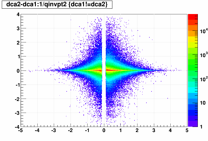
Zooming in the axis ranges a bit, and then limiting the histogam maximum makes clear that there are multiple bands:
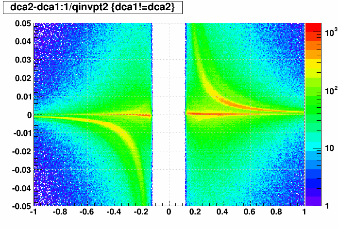
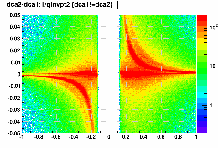
That there are bands, and where they are, makes sense. Accounting for energy loss in the track projection causes the direction of the shift to flip with charge of the track, and different materials with different densities and/or projection distances (e.g. at larger radii) will create different bands.
...But what doesn't make sense is why there are any positively charged tracks with negative ΔDCA (or negatively charged with positive ΔDCA)?!?
Multiplying ΔDCA by q*pT2 ≡ Δscaled makes the bands nearly flat, allowing us a metric to see where material is that produces these bands:
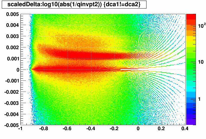
For some sense of scale, a Δscaled value of 0.0015 means that a pT = 316 MeV/c track sees a 150 μm ΔDCA, or a pT = 1 GeV/c track sees a 15 μm ΔDCA.
Accounting for energy loss means that added material will cause Δscaled to be shifted (biased) positively by an amount related to the amount of material added. On top of that there is a smearing, but I'm not 100% sure what that is (does Sti's projection include some additional random factor for multiple coulomb scatter??).
Here are Δscaled vs. z @ r~0 cm for various material differences, where bin contents are plotted logarithmicly and normalized by the number of tracks at each z (to reduce visual effects due simply to statistics). This normalization means that the content reflects the fraction of all tracks at each z with that Δscaled value. The histogram content ranges are restricted to [0.0015,0.015] to remove the statistically insignificant, while still highlighting small details. For example, solid red means that at least 1.5% of all tracks at that z have that value of dscaled, and green means ~0.5% of all tracks at that z.
Nothing → PXL:

Nothing → PXL+IST and PXL → PXL+IST:


Nothing → PXL+IST+SSD and PXL+IST → PXL+IST+SSD:


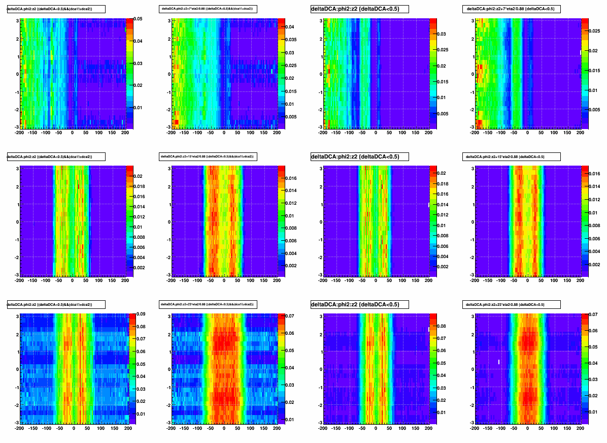
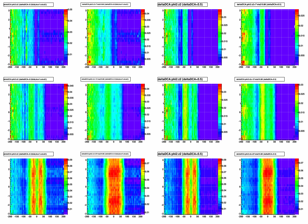
Here are the similar φ-dependence plots. I'm showing only small versions of the first 4 because the first 3 are all rather featureless in the φ projection, while the 4th conveys nothing more than the 5th, which shows some fascinating features!
Nothing → PXL, Nothing → PXL+IST, PXL → PXL+IST, Nothing → PXL+IST+SSD, and PXL+IST → PXL+IST+SSD:


The inclusion of SSD seems to have some rather interesting features:
Nothing → PXL:

Nothing → PXL+IST and PXL → PXL+IST:


Nothing → PXL+IST+SSD and PXL+IST → PXL+IST+SSD:


_______________
-Gene
This is specifically for the state of the HFT materials as they were in SL14d for the April 2014 preview production. We will likely modify and improve upon these representations of the HFT geometry.
_______
Materials are added separately for PXL, IST, and SSD.
Observations of note:
- PXL sensitive (thin) material appears not to be centered around z=0, but rather at approximately [0,+15cm].
- The rest of the PXL materials seem reasonably placed.
- PXL material includes something at phi near 0 and ±pi for all positive z.
- IST material near z=0 appears comparable to PXL material at large negative z.
- SSD is the largest material contribution of the three.
- SSD materials at large ±z seem to be at specific phi (neither specifically horizontal nor vertical locations).
- All materials' effects are in the "hundreds of microns" range, nearing 1 mm with the fully summed materials.
Plots:
As a metric of the effect on track projections with the accounting of material, I used <|ΔDCA|> for global tracks which had at least 25 TPC hits, 0.3 < pT < 2.0 GeV/c, and the 2D DCA to the BeamLine was within 2 cm (i.e. the track did not need to be close to a primary vertex, though the "beamline" was defined by the highest ranked primary vertex (x,y)). For the plots which use non-zero radius, I only made a correction to the z location via z + radius * (η/0.88), which is reasonable to first order for the precision of the plots I have made (the radii I used are only meant to be rough approximations for where material might be anyhow). Some additional explanations follow in the outline of what is presented:
There are a lot of plots, so please read the explanations first...
- Four sets of 12 plots:
- <|ΔDCA|> when incremental materials going from (3 rows):
- Nothing → PXL
- PXL → PXL+IST
- PXL+IST → PXL+IST+SSD
- <|ΔDCA|> for summed materials going from (3 rows):
- Nothing → PXL
- Nothing → PXL+IST
- Nothing → PXL+IST+SSD
- Same as A, but plot contents are logarithmically colored
- The logarithmic scale helps obviate small-scale effects
- Same as B, but plot contents are logarithmically colored
- <|ΔDCA|> when incremental materials going from (3 rows):
- Four columns:
- <|ΔDCA|> vs. φ,z @ r~0, excluding tracks which were unaffected (ΔDCA ≡ 0)
- Exclusion of such tracks is meant to convey the affect on tracks that actually go through the material
- <|ΔDCA|> vs. φ,z @ r~7,15,23 cm respectively for the 3 rows of each of the 4 sets, excluding tracks which were unaffected
- Projecting to such radii is meant to convey more realistically the z positions of the actual materials
- <|ΔDCA|> vs. φ,z @ r~0, for all tracks, regardless of whether they were unaffected
- Inclusion of such tracks is meant to convey the total affect on tracking in general for analyses/calibrations
- <|ΔDCA|> vs. φ,z @ r~7,15,23 cm respectively for the 3 rows of each of the 4 sets, for all tracks, regardless of whether the were unaffected
- <|ΔDCA|> vs. φ,z @ r~0, excluding tracks which were unaffected (ΔDCA ≡ 0)
(Note: images may be opened in another browser window/tab for higher resolution, or clicked on for PDF versions. All distance units are [cm])

_______________
Let's take a closer look at the ΔDCA distributions (instead of their means)...I will exclude all unaffected tracks (ΔDCA ≡ 0)...
Here is ΔDCA vs. q/pT:
Zooming in the axis ranges a bit, and then limiting the histogam maximum makes clear that there are multiple bands:
That there are bands, and where they are, makes sense. Accounting for energy loss in the track projection causes the direction of the shift to flip with charge of the track, and different materials with different densities and/or projection distances (e.g. at larger radii) will create different bands.
...But what doesn't make sense is why there are any positively charged tracks with negative ΔDCA (or negatively charged with positive ΔDCA)?!?
Multiplying ΔDCA by q*pT2 ≡ Δscaled makes the bands nearly flat, allowing us a metric to see where material is that produces these bands:
For some sense of scale, a Δscaled value of 0.0015 means that a pT = 316 MeV/c track sees a 150 μm ΔDCA, or a pT = 1 GeV/c track sees a 15 μm ΔDCA.
Accounting for energy loss means that added material will cause Δscaled to be shifted (biased) positively by an amount related to the amount of material added. On top of that there is a smearing, but I'm not 100% sure what that is (does Sti's projection include some additional random factor for multiple coulomb scatter??).
Here are Δscaled vs. z @ r~0 cm for various material differences, where bin contents are plotted logarithmicly and normalized by the number of tracks at each z (to reduce visual effects due simply to statistics). This normalization means that the content reflects the fraction of all tracks at each z with that Δscaled value. The histogram content ranges are restricted to [0.0015,0.015] to remove the statistically insignificant, while still highlighting small details. For example, solid red means that at least 1.5% of all tracks at that z have that value of dscaled, and green means ~0.5% of all tracks at that z.
Nothing → PXL:
Nothing → PXL+IST and PXL → PXL+IST:
Nothing → PXL+IST+SSD and PXL+IST → PXL+IST+SSD:
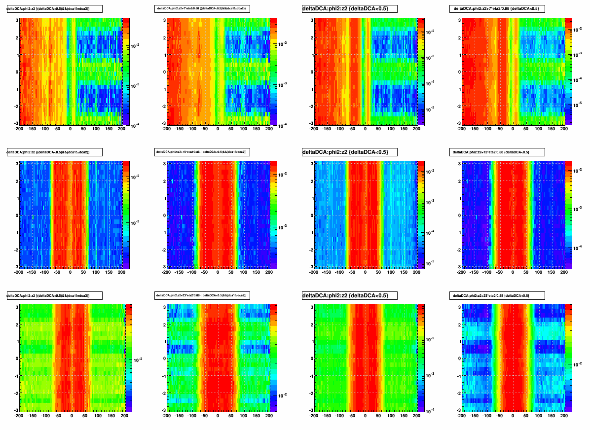
Here are the similar φ-dependence plots. I'm showing only small versions of the first 4 because the first 3 are all rather featureless in the φ projection, while the 4th conveys nothing more than the 5th, which shows some fascinating features!
Nothing → PXL, Nothing → PXL+IST, PXL → PXL+IST, Nothing → PXL+IST+SSD, and PXL+IST → PXL+IST+SSD:
The inclusion of SSD seems to have some rather interesting features:
- Something φ-segmented is introduced for |z|>~50 cm with either significant material or longer projection (at larger radius) which affects ~0.5% of all tracks!
- Something else etween some of these first segments is a different material with even larger effect, but only at a few φ and localized to z~0!
- Both of thse first two observed materials feature a kink in Δscaled at φ~+π/2 (straight up).
- IST and PXL contributions around z~0 become less visible because the same tracks (presumably) go through SSD materials, which has a greater effect.
- There is a band across all z, at rather specific φ, with a negative Δscaled. This means that material in the PXL+IST configuration gets missed due to the inclusion of the SSD!
Nothing → PXL:
Nothing → PXL+IST and PXL → PXL+IST:
Nothing → PXL+IST+SSD and PXL+IST → PXL+IST+SSD:
_______________
-Gene
Groups:
- genevb's blog
- Login or register to post comments