The mean of the Landau distribution is undefined
Updated on Sat, 2018-04-07 13:28. Originally created by lisa on 2018-03-30 15:15.
One hears that the mean of the Landau distribution is undefined. Hey, if it says so on Wikipedia, it must be right!
Still, say you sample a Landau distribution N times, getting N numbers. Any finite set of numbers has a mean, right? Sure. But that's not the point. I want to know whether summing up nMIP (calibrated ADC value) gives an estimate of the multiplicity in the EPD. Conclusions are given at the bottom of the page.
As a note, I don't know whether the numerical Landau distribution implemented in root is 100% correct (apparently that's nontrivial), but I do know that it describes the EPD ADC distribution quite well, and it is the mathematical formula behind the energy loss in a scintillator. So, we're assuming it's the "truth."
Consider the following root macro, which calculates the average of a Gaussian distribution, when sampled 10^N times
void AverageOfGauss(){
TRandom3 *ran = new TRandom3;
ran->SetSeed();
TProfile* GaussMean = new TProfile("GaussMean","GaussMean",8,2.5,10.5);
for (int exponent=3; exponent<10; exponent++){
cout << "Exponent is " << exponent << endl;
int ntry = pow(10.0,exponent);
for (int i=1; i<ntry; i++){
GaussMean->Fill(exponent,ran->Gaus(1.0,0.15));
}
}
GaussMean->Draw();
}
It makes the following pictures, where N is on the x-axis: (the two pictures are the same, just blown up scale on the second one):

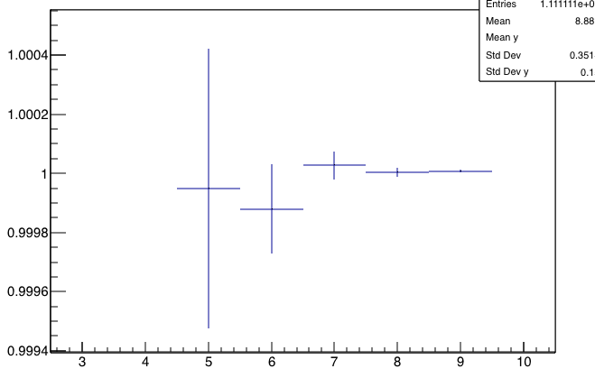
You see that
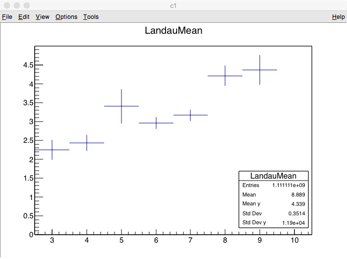
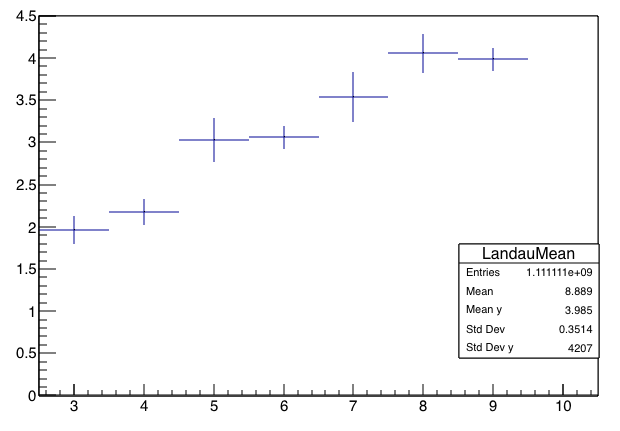
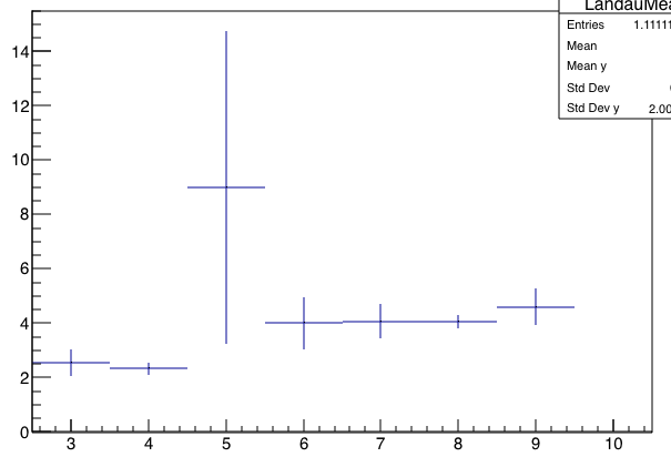
Now let's do the same thing for Landau:
void AverageOfLandau(){
TRandom3 *ran = new TRandom3;
ran->SetSeed();
TProfile* LandauMean = new TProfile("LandauMean","LandauMean",8,2.5,10.5);
for (int exponent=3; exponent<10; exponent++){
cout << "Exponent is " << exponent << endl;
int ntry = pow(10.0,exponent);
for (int i=1; i<ntry; i++){
LandauMean->Fill(exponent,ran->Landau(1.0,0.15));
}
}
LandauMean->Draw();
}
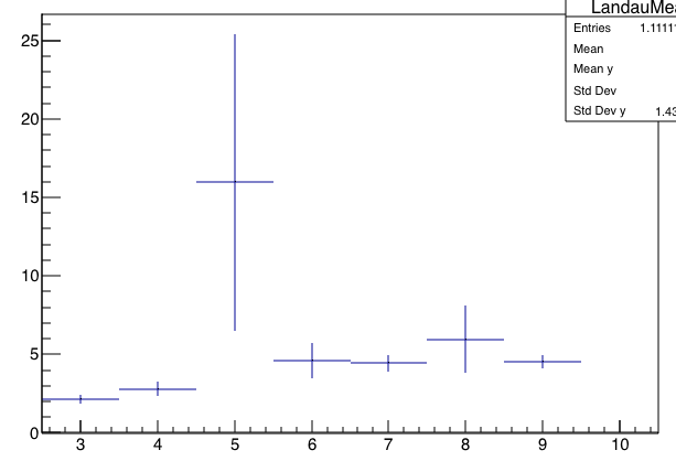
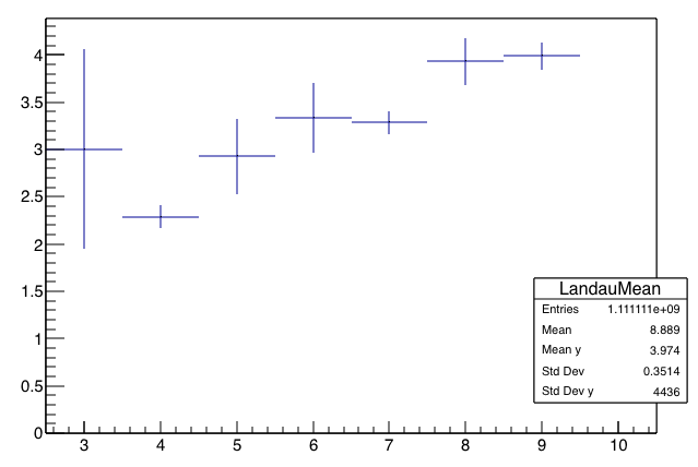
Here's what you get. These are six different runs of the code above:
.png)
Observations:
Implications:
Additional details:
The multiplicative scale depends on WID/MPV, as one might expect. In the plots above, WID/MPV=0.15. Below is an example where WID/MPV=0.3"
A final detail: In principle, the Landau probability is finite even for "negative energy loss." Naturally, the lowest we can see is zero. If I redo the calculation, but say "if (x<0) x=0;", it makes no difference at all for WID/MPV=0.15 and essentially none for 0.3, because in those cases the probability density for x<0 is small.
Still, say you sample a Landau distribution N times, getting N numbers. Any finite set of numbers has a mean, right? Sure. But that's not the point. I want to know whether summing up nMIP (calibrated ADC value) gives an estimate of the multiplicity in the EPD. Conclusions are given at the bottom of the page.
As a note, I don't know whether the numerical Landau distribution implemented in root is 100% correct (apparently that's nontrivial), but I do know that it describes the EPD ADC distribution quite well, and it is the mathematical formula behind the energy loss in a scintillator. So, we're assuming it's the "truth."
Consider the following root macro, which calculates the average of a Gaussian distribution, when sampled 10^N times
void AverageOfGauss(){
TRandom3 *ran = new TRandom3;
ran->SetSeed();
TProfile* GaussMean = new TProfile("GaussMean","GaussMean",8,2.5,10.5);
for (int exponent=3; exponent<10; exponent++){
cout << "Exponent is " << exponent << endl;
int ntry = pow(10.0,exponent);
for (int i=1; i<ntry; i++){
GaussMean->Fill(exponent,ran->Gaus(1.0,0.15));
}
}
GaussMean->Draw();
}
It makes the following pictures, where N is on the x-axis: (the two pictures are the same, just blown up scale on the second one):


You see that
- the result converges to the "right" answer
- the statistical errorbars calculated by root go as 1/sqrt(N) and also properly characterize the fluctuation and discrepancy from the right answer.
Now let's do the same thing for Landau:
void AverageOfLandau(){
TRandom3 *ran = new TRandom3;
ran->SetSeed();
TProfile* LandauMean = new TProfile("LandauMean","LandauMean",8,2.5,10.5);
for (int exponent=3; exponent<10; exponent++){
cout << "Exponent is " << exponent << endl;
int ntry = pow(10.0,exponent);
for (int i=1; i<ntry; i++){
LandauMean->Fill(exponent,ran->Landau(1.0,0.15));
}
}
LandauMean->Draw();
}
Here's what you get. These are six different runs of the code above:


.png)

Observations:
- The errorbars, which are "spread/sqrt(N)," usually considered "the uncertainty on the mean," do not go down smoothly with N. The spread of the sample grows on order of sqrt(N). Hence, the fractional uncertainty in the sum does not go down with increased number of samples being summed.
- The "mean" doesn't converge to any number. Indeed, the mean tends to grow with the number of samples, as the likelihood of picking up a large fluctuation in the long tail outweighs the fluctuations on the lower side.
Implications:
- "nMIP-weighted" analyses will be subject to huge fluctuations which will not be compensated by high statistics
- in "nMIP-weighted" procedures, errorbars based on 1/sqrt(N) will be wrong.
- At one point, I had claimed that one could "correct" for the Landau tail, in a "nMIP-weighted" eta distribution, simply by applying a multiplicative factor. The above plots tell me that this is not quite right. There is no unique factor. However, it gives a scale of the effect, and what the plots say is that for WID/MPV = 0.15, an "nMIP-weighted" multiplicity distribution will return a result that is ~2-4 times too high, for sampling between 1000 and 1,000,000,000 times.
- This is a pretty rough number and should not be used as a "correction factor", but at least it gives a scale. We are not looking at factors of 1000 here.
- even this "multiplicative factor" can have wild fluctuations, however, as can be seen above.
- I've shown before that this "multiplicative scale" depends on WID/MPV. See bottom of page.
- Inclusive analyses like dN/deta distributions (and even v2, if the event plane is determined by a different detector) need to be done with the fitting method.
- Where event information is needed from the EPD (like to obtain an event plane or centrality measure), "nMIP-weighted" analyses are the only option on the table (right?) but be aware of these large fluctuations.
- e.g. Define SumEpd = the sum of all the nMIP (equivalently, the sum of all the gain-corrected ADCs) in the EPD. Probably a large SumEpd is a higher multiplicity event than a small SumEpd, but the resolution is not trivial. And at some point, cutting in ever-finer bins (like % or sub-% in SumEpd) is meaningless.
- Fortunately, for the event-plane, one gets a measure of the resolution from the data itself. And don't despair! Keep in mind that the BBC has even worse fluctuations (since it is a little thinner scintillator and I believe fewer photons are captured per MIP), and an "nMIP_weighted" method was good enough to define reaction planes for several PRLs and a Nature paper ;-)
Additional details:
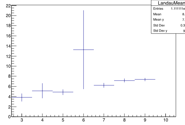
The multiplicative scale depends on WID/MPV, as one might expect. In the plots above, WID/MPV=0.15. Below is an example where WID/MPV=0.3"

A final detail: In principle, the Landau probability is finite even for "negative energy loss." Naturally, the lowest we can see is zero. If I redo the calculation, but say "if (x<0) x=0;", it makes no difference at all for WID/MPV=0.15 and essentially none for 0.3, because in those cases the probability density for x<0 is small.
»
- lisa's blog
- Login or register to post comments
