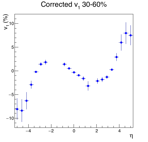
v1 analysis of charged particles in Au+Au 27 GeV
Updated on Thu, 2018-06-07 12:15. Originally created by lisa on 2018-06-03 21:45.
Executive summary:
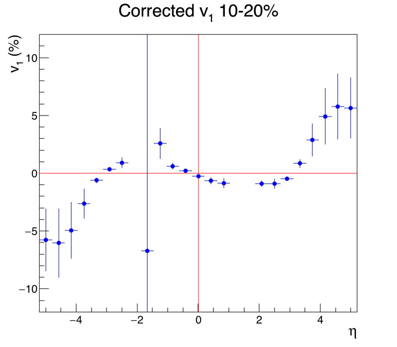
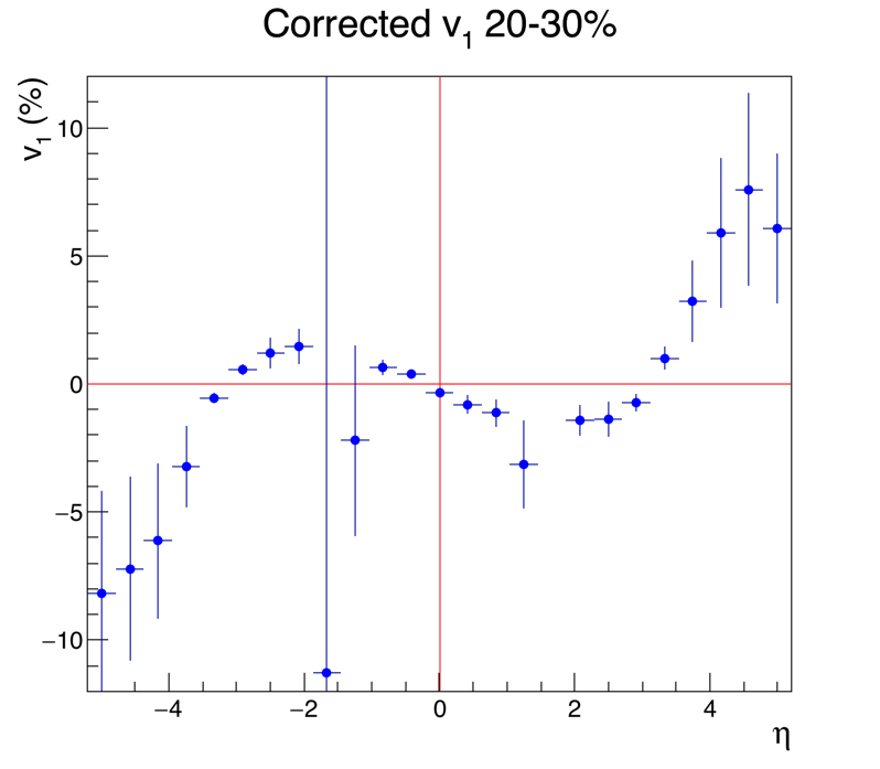
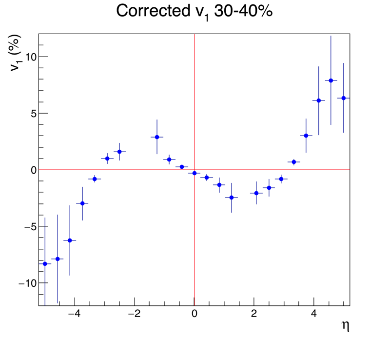
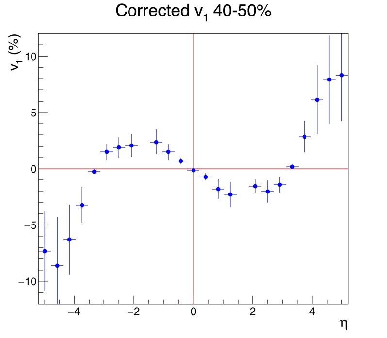
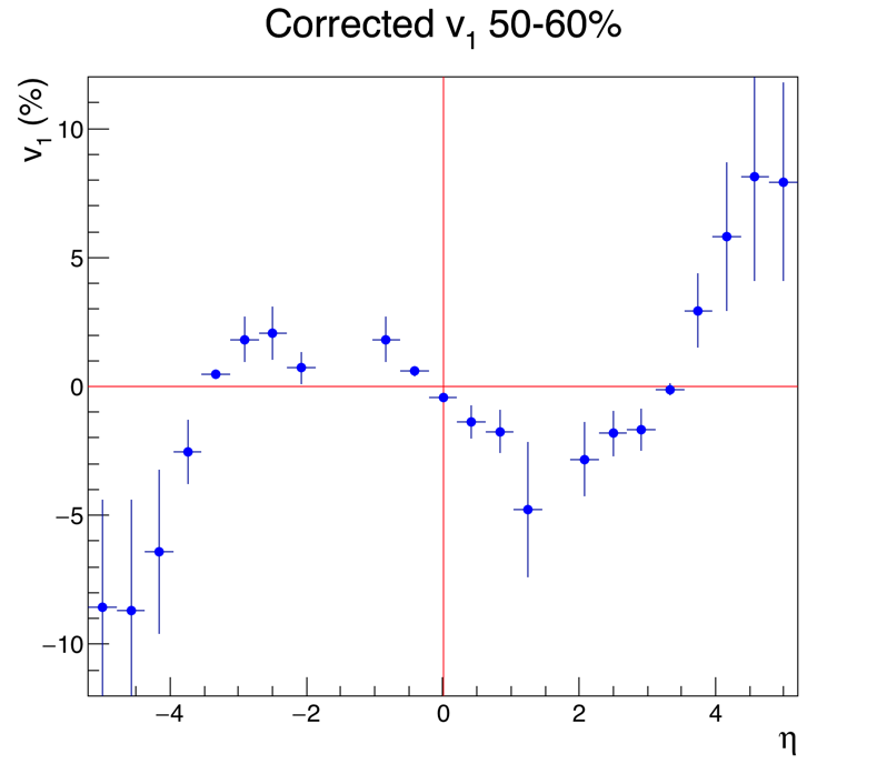
This is a first analysis of v1 in Au+Au collisions at 27 GeV, taken in 2018. At some point I may have time to post captions and explanations of all the plots, but if you've been following my 10N other EPD posts, you can figure out what they are.
Click here to go to the bottom for an update made 7 June 2018.
.png)
.png)
Update 7 June 2018
During my presentation to bulkcorr on 6 June 2018, Gang suggested that the optimal ring weights probably mirror almost exactly the v1-versus-eta graph, since it is v1 that gives the anisotropy. This is reasonable, but I'll point out that the flux (yield) at a given eta will also affect the sensitivity of that eta region, to the event plane. So, it may not be so simple. Let's take a look:
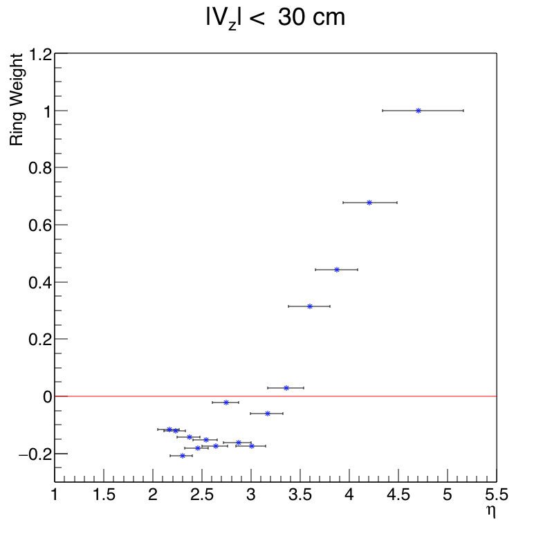
Figure - Optimized ring weight (from rightmost column of table 1 on this page) versus eta of the ring. The eta ranges indicated by the "errorbars" correspond to the finite size of the tile, and the fact that the primary vertex ranges from -30 cm to +30 cm in my analysis.
Yep, that very much resembles the measured v1! In sign, in zero-crossing-point, and in relative amplitude, it mirrors v1 very well.
(BTW, there is one weight (for ring 9) that seems "out-of-place" relative to his neighbors. As I noted here, I believe this is a fit fluctuation; don't worry about it.)
Something else: as the caption to the figure says, there is a range of eta corresponding to any tile. This is driven by two things:
Let's make a couple of plots that illustrate the relative importance of Vz fluctuations and finite tile size.
Here is the same figure as above, except if the primary vertex is in the exact center of the TPC (Vz=0). The y-coordinates are the same as above, just for illustration:

The same as the plot above, except I consider only if Vz=0.0. It shows the eta range sampled by tiles in the 16 rings (Ring 1 on the right and Ring 16 on the left). There is no overlap. In this figure, the finite range is driven entirely by the finite size of the tile.
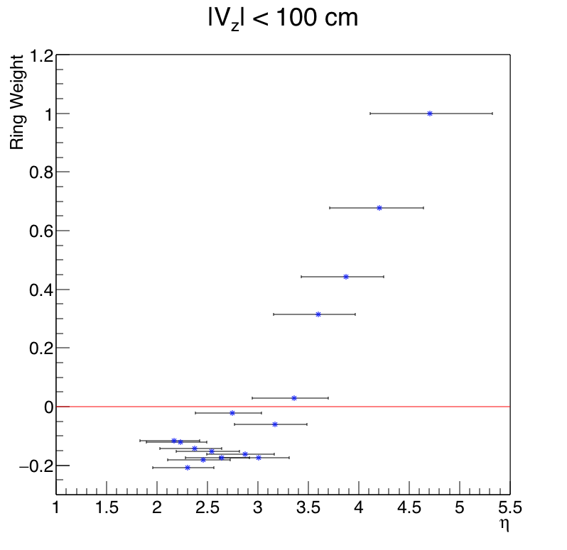
The same as the plots above, except I look at the extremes where Vz=-100 to Vz=+100 cm. Especially for the outer tiles (low eta), the primary vertex fluctuations drive the range of eta sampled by the tiles; their finite size is irrelevant.
I hesitate to show these plots, because somebody is going to say "oh, if we have a primary vertex distribution that is wide, then a tile will sample a huge range in eta, and everything will get washed out." Yes, somebody is going to say that, but don't let it be you, okay? Looking at the code above, you'll see that I account for the primary vertex position in every event. So it's just the finite size that generates some limits, and these limits are even smaller than the ones in the second-to-last plot above.
However, it does make the point that I should make weights that depend on eta, not ring. (Ring is okay if I only look at events from Vz~0, because then the ring-to-eta mapping is 1:1.) Because the anisotropy is driven by physics, and physics cares about eta, not ring. Gang made this point yesterday, and I agree.
Executive summary:
This is a first analysis of v1 in Au+Au collisions at 27 GeV, taken in 2018. At some point I may have time to post captions and explanations of all the plots, but if you've been following my 10N other EPD posts, you can figure out what they are.
Click here to go to the bottom for an update made 7 June 2018.
Update 7 June 2018
During my presentation to bulkcorr on 6 June 2018, Gang suggested that the optimal ring weights probably mirror almost exactly the v1-versus-eta graph, since it is v1 that gives the anisotropy. This is reasonable, but I'll point out that the flux (yield) at a given eta will also affect the sensitivity of that eta region, to the event plane. So, it may not be so simple. Let's take a look:
Figure - Optimized ring weight (from rightmost column of table 1 on this page) versus eta of the ring. The eta ranges indicated by the "errorbars" correspond to the finite size of the tile, and the fact that the primary vertex ranges from -30 cm to +30 cm in my analysis.
Yep, that very much resembles the measured v1! In sign, in zero-crossing-point, and in relative amplitude, it mirrors v1 very well.
(BTW, there is one weight (for ring 9) that seems "out-of-place" relative to his neighbors. As I noted here, I believe this is a fit fluctuation; don't worry about it.)
Something else: as the caption to the figure says, there is a range of eta corresponding to any tile. This is driven by two things:
- The finite size of the tile: a particle hitting at the innermost edge (i.e. smallest radius from the beamline) of the tile has a high eta, and a particle hitting at the outermost edge has a low eta.
- Fluctuations in the primary vertex position. If the primary vertex is very far away from the EPD wheel, then a tile will see higher eta than he will for events when the primary vertex is close to the wheel.
In the above, PV is a TVector3 of the primary vertex. As I've discussed before in the EPD group, this is the best you can do. We do not have tracking or charge sign or momentum information in the EPD, so we assume a straight line trajectory between primary vertex and the struck tile. (Artifacts from this assumption need to be evaluated in simulation.) Not every particle is going to strike the center of the tile (though we do have a TileCenter() method), so when making a distribution (or average) as a function of eta, you ought to sample the face of the tile, as RandomPointOnTile() does. If you think about it, it's kind of obvious. If it is obvious to you, great! If not, then it can be a long discussion, and I don't have time for that right now.TVector3 pos = mEpdGeom->RandomPointOnTile(epdHit->id());
TVector3 StraightLine = pos - PV;
double eta = StraightLine.Eta();
Let's make a couple of plots that illustrate the relative importance of Vz fluctuations and finite tile size.
Here is the same figure as above, except if the primary vertex is in the exact center of the TPC (Vz=0). The y-coordinates are the same as above, just for illustration:
The same as the plot above, except I consider only if Vz=0.0. It shows the eta range sampled by tiles in the 16 rings (Ring 1 on the right and Ring 16 on the left). There is no overlap. In this figure, the finite range is driven entirely by the finite size of the tile.
The same as the plots above, except I look at the extremes where Vz=-100 to Vz=+100 cm. Especially for the outer tiles (low eta), the primary vertex fluctuations drive the range of eta sampled by the tiles; their finite size is irrelevant.
I hesitate to show these plots, because somebody is going to say "oh, if we have a primary vertex distribution that is wide, then a tile will sample a huge range in eta, and everything will get washed out." Yes, somebody is going to say that, but don't let it be you, okay? Looking at the code above, you'll see that I account for the primary vertex position in every event. So it's just the finite size that generates some limits, and these limits are even smaller than the ones in the second-to-last plot above.
However, it does make the point that I should make weights that depend on eta, not ring. (Ring is okay if I only look at events from Vz~0, because then the ring-to-eta mapping is 1:1.) Because the anisotropy is driven by physics, and physics cares about eta, not ring. Gang made this point yesterday, and I agree.
»
- lisa's blog
- Login or register to post comments